mald_filt <- readRDS("data/tucker2019/mald_1_1.rds") |>
filter(RT > 34)36 Interactions in regression: one categorical and one numeric predictor


In Chapter 35, you learned how to include and interpret interactions between two categorical predictors: we modelled mean f0 in female vs male speakers in informal vs polite attitude. In this chapter, we will look at a model with an interaction between a categorical and a numeric predictor instead. Interactions between categorical and numeric predictors work on the same principles of interactions between two categorical predictors, but it is worth going through an example. We will revisit the model of reaction times from Chapter 31, but this time we will model RTs based on both mean phoneme-level Levenshtein distance and word type (real vs non-real).
36.1 The data
As usual, let’s attach the necessary packages and read the data. We filter RTs to include only values above 34 ms, as we have done in Chapter 31.
library(tidyverse)
theme_set(theme_light())
library(brms)
library(posterior)
library(tidybayes)
library(ggdist)We want to answer the following research question:
Does the effect of Levenshtein distance on RTs differ in real and non-real words?
To address this question we will need to model an interaction between distance and word type. Before we move onto modelling, let’s plot the data. Figure 36.1 shows a scatter plot with mean phoneme-level Levenshtein distance on the x-axis and logged reaction times on the y-axis. The plot also includes two regression lines: one for real words (in green) and one for non-real words (in orange).
Code
mald_filt |>
  ggplot(aes(PhonLev, RT_log)) +
  geom_point(alpha = 0.05) +
  geom_smooth(aes(colour = IsWord), method = "lm") +
  scale_color_brewer(palette = "Dark2") +
  labs(x = "Levenshtein distance", y = "RT (ms)")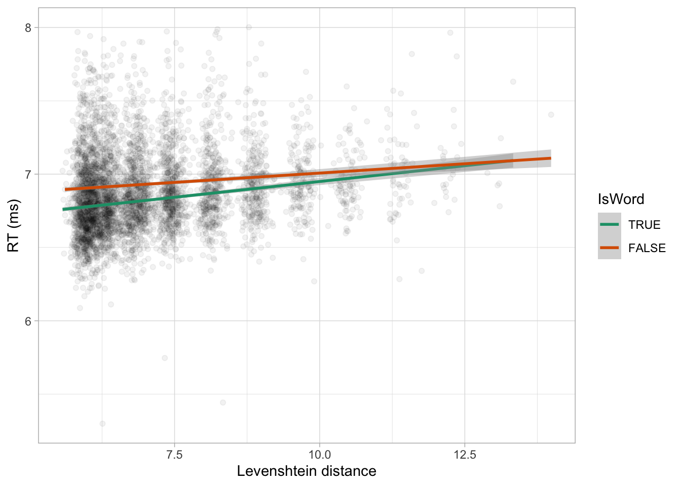
From glancing at the plot, it looks like the regression line is steeper in real words relative to non-real words, although they do end up overlapping at higher Levenshtein distance, thus potentially indicating a ceiling effect of Levenshtein distance. Independent of the reason behind this pattern (which statistics per se cannot answer), we can run a regression model to quantify differences.
36.2 One categorical and one numeric predictor (no interaction)
Let’s start by figuring out what the model mathematical formula looks like. First, let’s build the formula without the interaction term.
\[\begin{aligned} RT_i & \sim LogNormal(\mu_i, \sigma)\\ \mu_i & = \beta_0 + \beta_1 \cdot l_i + \beta_2 \cdot w_i\\ \end{aligned}\]
\(l\) is Levenshtein distance and \(w\) is the indicator variable for
IsWord. \(w=0\) isTRUEand \(w=1\) isFALSE. (The reference level ofIsWordisTRUE.)\(\beta_0\) is the intercept, i.e. the mean logged RTs (logged because it is a log-normal model) when
PhonLevis 0 andIsWordis the reference level,TRUE.\(\beta_1\) is the difference in outcome (i.e. mean logged RTs) for each unit increase of
PhonLev, while controlling forIsWord.\(\beta_2\) is the difference in outcome when the word is a non-real word compared to when it is a real word, while controlling for
PhonLev.
Since there is no interaction between distance and word type, the effect of distance on RTs is estimated to be the same independent of which word type the observation comes from and vice versa, the effect of word type on RTs is estimated to be the same independent of the value of distance. Let’s run this model so we can inspect the estimates of the regression coefficients and plot the results to see what the estimated effects look like.
rt_lw <- brm(
  RT ~ PhonLev + IsWord,
  family = lognormal,
  data = mald_filt,
  cores = 4,
  seed = 1927,
  file = "cache/ch-regression-cat-num-rt_lw"
)
The model has three regression coefficients, as you would expect (in the following, the 80% CrI are shown).
fixef(rt_lw, probs = c(0.1, 0.9)) |> round(2) Estimate Est.Error Q10 Q90
Intercept 6.58 0.02 6.55 6.61
PhonLev 0.03 0.00 0.03 0.04
IsWordFALSE 0.11 0.01 0.10 0.12The
Interceptcorresponds to the logged RTs whenPhonLevis 0 andIsWordisTRUE. At 80% probability, the logged RTs in these conditions are between 6.55 and 6.61.According to the
PhonLevestimate, for each unit increase ofPhonLevthe logged RTs increase by 0.03 to 0.04 (when controlling for word type) at 80% confidence.IsWordFalseindicates that the logged RTs are 0.1 to 0.12 higher in non-words than in real words (when controlling for distance).
The estimated effect of PhonLev is the same in both real words (the reference level of IsWord) and in non-words. Vice versa, the estimated effect of IsWord is the same independent of the value of PhonLev. We can confirm this visually by plotting the expected values. For convenience, we use conditional_effects(). This time we use the method argument to tell the function to plot the linear predictor (method = "posterior_linpred") rather than the expected values (method = "posterior_epred"). We do this so that we can see the effects on the linear scale of logged RTs, rather than on the original scale (since we are using a log-normal model, which makes effects on the original scale log-linear rather than simply linear).
conditional_effects(rt_lw, "PhonLev:IsWord", method = "posterior_linpred")
conditional_effects(rt_lw, "IsWord:PhonLev", method = "posterior_linpred")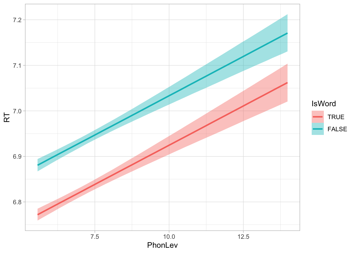
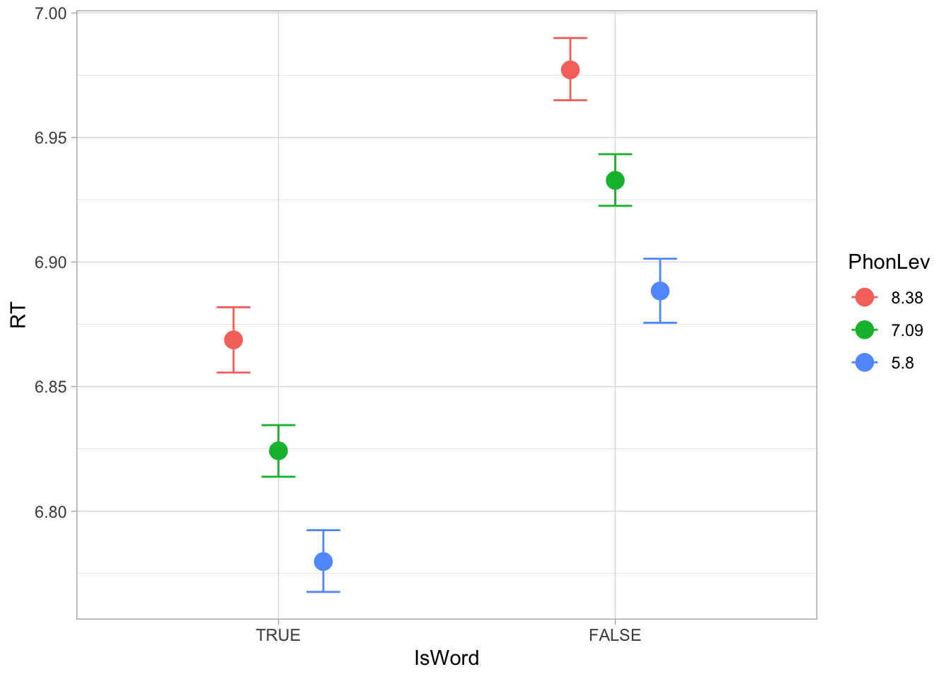
In Figure 36.2 (a), logged RT increase with greater mean phoneme-level Levenshtein distance in both real and non-words. If you look closely, you will also notice that the two regression lines are parallel. In other words, the slope of the lines is the same: this is because the model estimates a single effect of mean distance for both real and non-words. There is no other way this can be, because the model does not include an interaction between word type and distance. Conversely, if we look at Figure 36.2 (b), we can see that the effect of mean distance within real and non-words is the same in both word types. Note that conditional_effects() automatically picks “representative” values of the numeric predictor in this plot: by default, the representative values are the mean and mean \(\pm\) 1 SD of the observed values in the data for that predictor. If you compare, within each word type, the distances between the posterior logged RTs for the three values of distance, their distances are the same in both word types.
However, we have reasons to believe that the effects of word type and mean phoneme-level distance are not totally independent from each other. Why? Because this is the default assumption: from a linguistic point of view, we know that non-words behave differently from real words, so it makes sense to expect that the effect of phoneme-level distance might also be different. So what we really need is a model with an interaction between the two predictors. Note that we only fitted a model without an interaction for pedagogical reasons, but you should not fit a model without interactions if you intend to fit one with interactions.
36.3 One categorical and one numeric predictor in interaction
The model with an interaction between phoneme-level distance and word type can be represented with the following formula:
\[\begin{aligned} RT_i & \sim LogNormal(\mu_i, \sigma)\\ \mu_i & = \beta_0 + \beta_1 \cdot l_i + \beta_2 \cdot w_i + \beta_3 \cdot l_i \cdot w_i\\ \end{aligned}\]
Because of the interaction term \(\beta_3 \cdot l_i \cdot w_i\), now the effect of the each predictor depends on the value of the other. When distance \(l = 0\) and word type is non-word, the regression formula simplifies to \(\beta_0 + \beta_2\) (all terms with \(l\) are dropped). When distance \(l \neq 0\) and word type is non-word, then all terms are preserved and whatever value \(l\) takes is plugged in: \(\beta_0 + \beta_1 \cdot l_i + \beta_2 + \beta_3 \cdot l_i\).
The R syntax for interactions between predictors of different type is the same as with two categorical predictors: you include an interaction term by adding the two predictors separated by a colon, like PhonLev:IsWord. We have also seen the syntactic sugar * which automatically includes the main coefficients and the interaction term, but for clarity we use the full syntax here.
rt_lw_int <- brm(
  # Equivalent: RT ~ PhonLev * IsWord
  RT ~ PhonLev + IsWord + PhonLev:IsWord,
  family = lognormal,
  data = mald_filt,
  cores = 4,
  seed = 1927,
  file = "cache/ch-regression-cat-num-rt_lw_int"
)
Now that we have included an interaction, the interpretation of the PhonLev and IsWordFALSE coefficients changes.
fixef(rt_lw_int, probs = c(0.1, 0.9)) |> round(2) Estimate Est.Error Q10 Q90
Intercept 6.52 0.03 6.48 6.56
PhonLev 0.04 0.00 0.04 0.05
IsWordFALSE 0.23 0.04 0.18 0.29
PhonLev:IsWordFALSE -0.02 0.01 -0.02 -0.01The
Interceptis still the logged RTs when phoneme-level distance is 0 and the word is real, but you will notice that the estimate is slightly different now. This is common when including an interaction between predictors. Since the effects of each predictor are allowed to differ depending on the value of the other predictor, the intercept might be affected.Now, the
PhonLevcoefficient is the effect ofPhonLevwhen the word is real. In other words, the estimate of this coefficient applies exclusively to real words. Why real words? Because that’s the reference level ofIsWord. According to the model, for each unit increase of phoneme-level distance in real words, logged RTs increase by 0.04 to 0.05 (at 80% probability). This is a slightly larger difference than that estimated by the model without the interaction.IsWordFALSEtells us the difference between non-words and real words when phoneme-level distance is 0. Why 0? Because that’s the “default” value of a numeric predictor. Non-words elicit logged RTs that are 0.18 to 0.29 longer than real words, when distance is 0. This difference is much larger than the one suggested by the model without an interaction.PhonLev:IsWordFALSEis the coefficient of the interaction term. This coefficient tells us how the effect ofPhonLevdiffers in non-words vs real words. In other words, it tells us what we need to add or subtract to the phoneme-level distance effect of real words to get that effect in non-words. According to the model, the effect of distance in non-words on logged RTs is between 0.01 and 0.02 units smaller than the effect in real words, at 80% confidence. This is because the 80% CrI of the posterior distribution of the coefficient is [-0.02, -0.01].
So what is the effect of phoneme-level distance in non-words? Easy, we can compute that using the posterior draws of the PhonLev and PhonLev:IsWordFALSE coefficients. We simply sum them to obtain the effect of mean distance on logged RTs when the word is a non-word.
rt_lw_int_draws <- as_draws_df(rt_lw_int) |>
  mutate(
    # Remember to use backticks `` with column names that have colons.
    PhonLev_false = b_PhonLev + `b_PhonLev:IsWordFALSE`
  )

quantile2(rt_lw_int_draws$PhonLev_false, probs = c(0.1, 0.9)) |> round(2)
q10 q90
0.02 0.03 The 80% CrI of the posterior draws of the effect of distance in non-words is between 0.02 and 0.03. Compare it with the effect in real words, [0.04, 0.05]. The slope of the regression line of the effect of phoneme-level distance on logged RTs is thus less steep in non-words than in real words. How less steep is quantified by the PhonLev:IsWordFALSE coefficient. How does all this look like? Let’s plot the posterior draws of the linear predictor using conditional_effects().
conditional_effects(rt_lw_int, "PhonLev:IsWord", method = "posterior_linpred")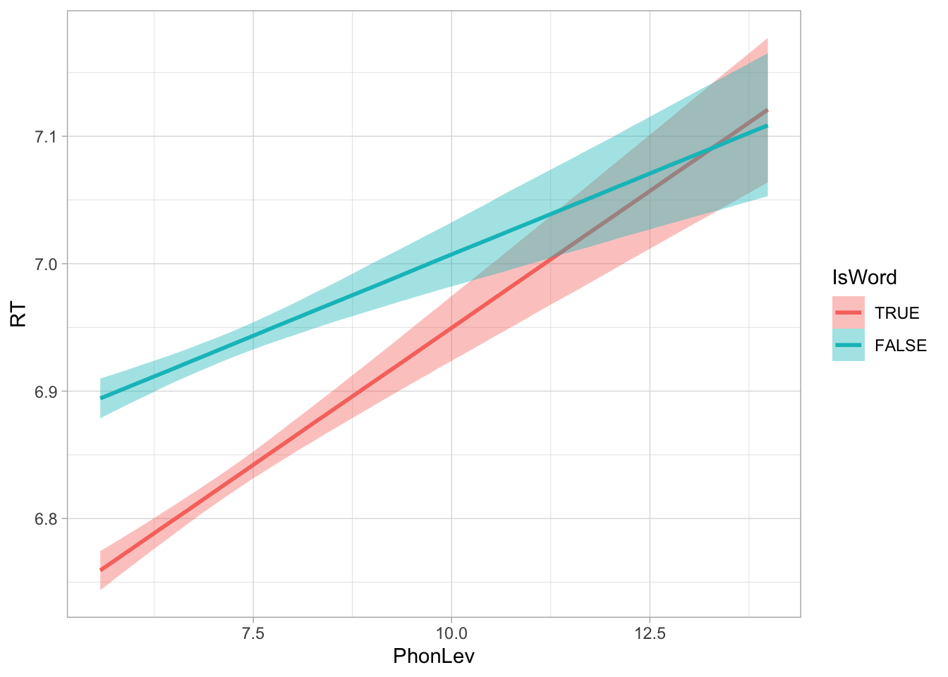
Figure 36.3 shows the regression lines for real and non-words. The line is steeper in real words than in non-words. In other words, for each unit increase of phoneme-level distance, the logged RTs increase more in real than in non-words. Let’s plot the expected values now, but instead of using conditional_effects(), let’s use epred_draws(). First, we need the grid:
epred_grid <- expand_grid(
  PhonLev = seq(min(mald_filt$PhonLev), max(mald_filt$PhonLev), by = 0.1),
  IsWord = c("TRUE", "FALSE")
) |>
  mutate(
    # We convert IsWord to factor so we can specify the order of the levels.
    IsWord = factor(IsWord, levels = c("TRUE", "FALSE"))
  )
Now, we can calculate the expected values.
rt_lw_int_epred <- epred_draws(
  rt_lw_int,
  epred_grid
)

rt_lw_int_epred
For plotting effects of numeric predictors, we need to calculate the mean and lower and upper limits of the credible interval.
rt_lw_int_epred_cri <- rt_lw_int_epred |>
  summarise(
    mean = mean(.epred),
    lower = quantile2(.epred, probs = 0.025),
    upper = quantile2(.epred, probs = 0.975)
  )
Finally, we can plot the expected values.
rt_lw_int_epred_cri |>
  ggplot(aes(PhonLev, mean)) +
  geom_ribbon(aes(ymin = lower, ymax = upper, fill = IsWord), alpha = 0.2) +
  geom_line(aes(colour = IsWord), linewidth = 1) +
  scale_fill_brewer(palette = "Dark2") +
  scale_colour_brewer(palette = "Dark2") +
  labs(x = "Phoneme-level distance", y = "Expected RTs (ms)", colour = "Real word?", fill = "Real word?")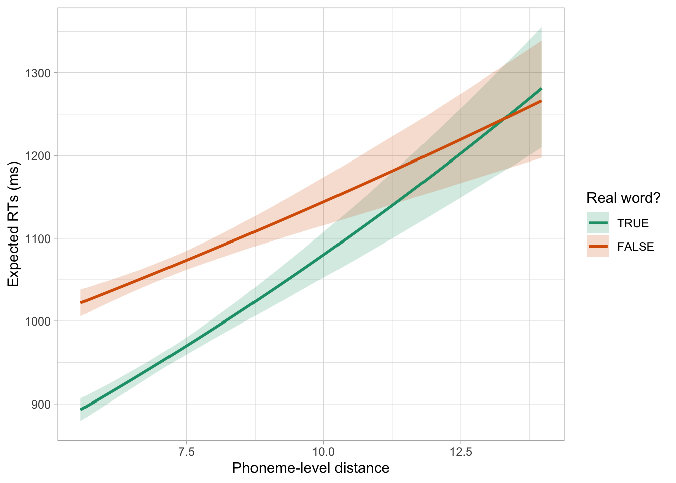
36.4 Calculating posterior draws at specific predictor values
With categorical/numeric interactions, it is often useful to calculate and report differences (aka comparisons) between the levels of the categorical predictor at different values of the numeric predictor. There isn’t a specific recipe to follow when it comes to calculating specific comparisons: it depends on the research question/hypothesis. Here, I illustrate how to calculate specific comparisons using three values of mean phoneme-level distance based on the range of values in the data. We can use 7, 10 and 12. From Figure 36.4, we should see a decreasing difference in logged RTs between non- and real words from distance 7 to 10 to 12.
We can calculate this difference using the posterior draws (and plugging in 7, 10, 12 in the regression formula) or use linpred_draws(). I will show you the former and you will do the latter as an exercise below. Before we get to the code, answer the following question.
The following code calculates the posterior draws of the linear predictor when distance is 7, 10, 12. Then, it gets the posterior draws of the difference between non-words and real words at those values of phoneme-level distance.
rt_lw_int_draws <- rt_lw_int_draws |>
  mutate(
    # Posterior draws of the linear predictor
    rt_log_7_true = b_Intercept + b_PhonLev * 7,
    rt_log_7_false = b_Intercept + b_PhonLev * 7 + b_IsWordFALSE + `b_PhonLev:IsWordFALSE` * 7,
    rt_log_10_true = b_Intercept + b_PhonLev * 10,
    rt_log_10_false = b_Intercept + b_PhonLev * 10 + b_IsWordFALSE + `b_PhonLev:IsWordFALSE` * 10,
    rt_log_12_true = b_Intercept + b_PhonLev * 12,
    rt_log_12_false = b_Intercept + b_PhonLev * 12 + b_IsWordFALSE + `b_PhonLev:IsWordFALSE` * 12,

    # Posterior draws of the difference
    rt_log_7 = rt_log_7_false - rt_log_7_true,
    rt_log_10 = rt_log_10_false - rt_log_10_true,
    rt_log_12 = rt_log_12_false - rt_log_12_true,
  )

# Get 90% CrI of the differences
quantile2(rt_lw_int_draws$rt_log_7, probs = c(0.1, 0.9)) |> round(2)
q10 q90
0.10 0.12 quantile2(rt_lw_int_draws$rt_log_10, probs = c(0.1, 0.9)) |> round(2) q10 q90
0.03 0.08 quantile2(rt_lw_int_draws$rt_log_12, probs = c(0.1, 0.9)) |> round(2) q10 q90
-0.02 0.06 The just calculated 80% CrIs of the posterior draws indicate that, at 80% probability, the logged RTs of non-words are 0.1 to 0.12 longer than those of real words when mean phoneme-level distance is 7, 0.03 to 0.08 longer when mean distance is 10 and they are -0.02 shorter to 0.06 longer when mean distance is 12. Indeed, the difference between real and non-words decreases with increasing mean distance, to the point where with mean distance 12 it is even possible that logged RTs are slightly faster in non-words than in real words (note however that the CrI spans both negative and positive values, with the majority of the CrI being along positive values).
36.5 Ratio effects
Let’s go back to our initial research question, Does the effect of Levenshtein distance on RTs differ in real and non-real words? Since the model uses a log-normal family, it is more straightforward to answer the question using ratios rather than logged milliseconds (on the linear predictor scale, i.e. logged RTs) or milliseconds (on the response scale, i.e. RTs). As we’ve done in Chapter 31, ratios can be calculated by exponentiating the log differences.
# Real words
quantile2(exp(rt_lw_int_draws$b_PhonLev), probs = c(0.1, 0.9)) |> round(2)
q10 q90
1.04 1.05 # Non-words
quantile2(exp(rt_lw_int_draws$b_PhonLev + rt_lw_int_draws$`b_PhonLev:IsWordFALSE`), probs = c(0.1, 0.9)) |> round(2) q10 q90
1.02 1.03 At 80% probability, RTs increase by a factor of 1.04-1.05 for each unit increase of mean phoneme-level Levenshtein distance in real words, while in non-words they increase by a factor of 1.02-1.03. In percentages, that is a 4-5% increase in real words and a 2-3% increase in non-words. We can also calculate ratios for more than one unit increase: let’s say for example we want the ratio between RTs when distance is 12 and when it is 7, in real and non-words. First, we need the number of units: \(12-7=5\). So between distance 7 and 12 there is an increase of 5 units. Now we can obtain the ratio of RTs at Levenshtein distance 12 to RTs at Levenshtein distance 5 by multiplying the posterior draws of the relevant coefficients by 5. Note that for non-words we need to multiply both b_PhonLev and b_PhonLev:IsWordFalse.
# Real words
quantile2(exp(rt_lw_int_draws$b_PhonLev * 5), probs = c(0.1, 0.9)) |> round(2)
q10 q90
1.21 1.27 # Non-words
quantile2(exp(rt_lw_int_draws$b_PhonLev * 5 + rt_lw_int_draws$`b_PhonLev:IsWordFALSE` * 5), probs = c(0.1, 0.9)) |> round(2) q10 q90
1.11 1.17 The RTs increase by 21-27% from distance 7 to distance 12 in real words, but only by 11-17% in non-words, at 80% confidence.
36.6 Reporting
We fitted a Bayesian regression model using the brms package (Bürkner 2017) in R (R Core Team 2025). We used a log-normal distribution for the outcome variable, reaction times (RTs, milliseconds). We included mean phoneme-level Levenshtein distance and word type (real vs non-real word) as the regression predictors and their interaction. Word type was coded using the default R treatment contrasts, with real word set as the reference level. The model was fitted with four MCMC chains, each with 2000 iterations, of which 1000 for warm-up. The default brms priors were used. The models’ \(\hat{R}\) values were all approximately 1, indicating convergence. The bulk and tail Estimated Sample Size were sufficient and the trace plots suggest the chains have mixed well. The posterior predictive plot doesn’t indicate major deviations from the observed distribution. See Table 36.1 for the full regression coefficients table.
According to the model’s intercept, The 90% CrI of RTs is [647, 713] ms when phoneme-level distance is 0 (\(\beta\) = 6.52, SD = 0.03). For real words, each unit increase of phoneme-level distance increases RTs by a factor of 1.04-1.05 at 90% probability (\(\beta\) = 0.04, SD = 0.004). When distance is 0, non-real words elicit RTs that are 1.18-1.25 times longer than real words (\(\beta\) = 0.23, SD = 0.04). The 90% CrI of the interaction coefficient is [-0.03, -0.01] on the log scale. In other words, each unit increase of phoneme-level distance in non-words increases RTs by a factor of 1.02-1.03 at 90% confidence (cf with 1.04-1.05 in real words). These results suggest that the effect of phoneme-level distance differs in real and non-real words, the effect being somewhat weaker in non-real words.
While the research question focuses on the effect of phoneme-level distance in real and non-words (Does the effect of Levenshtein distance on RTs differ in real and non-real words?), we can approach the results from the point of view of comparing the RTs of real and non-words at different values of distance. Because of the negative interaction coefficient, the difference in RTs between real and non-words is larger at lower phoneme-level distance and, conversely, smaller at higher phoneme-level distance. For illustration, at phoneme-level distance = 7, RTs for non-words are 1.10-1.13 times longer than real words; at distance = 10, they are 1.03-1.09 longer; and at distance = 12, they are 0.97 times shorter to 1.07 times longer, at 90% probability.
Code
fixef(rt_lw_int) |> knitr::kable(digits = 2)| Estimate | Est.Error | Q2.5 | Q97.5 | |
|---|---|---|---|---|
| Intercept | 6.52 | 0.03 | 6.46 | 6.58 |
| PhonLev | 0.04 | 0.00 | 0.03 | 0.05 |
| IsWordFALSE | 0.23 | 0.04 | 0.15 | 0.31 |
| PhonLev:IsWordFALSE | -0.02 | 0.01 | -0.03 | -0.01 |