library(tidyverse)

eu_vot <- read_csv("data/egurtzegi2020/eu_vot.csv")
eu_vot28 More than two levels
![]()
Chapter 27 showed you how to fit a regression model with a categorical predictor. We modelled reaction times as a function of word type (real or nonce) from the MALD dataset (Tucker et al. 2019). The categorical predictor IsWord (word type: real or nonce) was included in the model using treatment contrasts: the model’s intercept is the mean of the first level and the “slope” is the difference between the second level and the first. In this chapter we will look at new data, Voice Onset Time (VOT) of Mixean Basque (Egurtzegi and Carignan 2020), to illustrate how to fit and interpret a regression model with a categorical predictor that has three levels, phonation (voiced, voiceless unaspirated, aspirated).
28.1 Mixean Basque VOT
The data egurtzegi2020/eu_vot.csv contains measurements of VOT from 10 speakers of Mixean Basque (Egurtzegi and Carignan 2020). Mixean Basque contrasts voiceless unaspirated, voiceless aspirated and voiced stops. Let’s read the data.
Based on our general knowledge of VOT, the VOT should increase from voiced to voiceless unaspirated to voiceless aspirated stops. We can use a Gaussian regression model to assess whether our expectations are compatible with the data. The eu_vot data has a voicing column that tells only if the stop is voiceless or voiced, but we need a column that further differentiates between unaspirated and aspirated voiceless stops. We can create a new column, phonation depending on the phone, using the case_when() function inside mutate().
case_when() works like an extended ifelse() function: while ifelse() is restricted to two conditions (i.e. when something is TRUE or FALSE), chase_when() allows you to specify many conditions. The general syntax for the conditions in case_when() is condition ~ replacement where condition is a matching statement and replacement is the value that should be returned when there is a match. In the following code, we use case_when() to match specific phones in the phone column and based on that we return voiceless, voiced or aspirated. These values are saved in the new column phonation. We also convert the VOT values from seconds to milliseconds by multiply the VOT by 1000 in a new column VOT_ms.
eu_vot <- eu_vot |>
  mutate(
    phonation = case_when(
      phone %in% c("p", "t", "k") ~ "voiceless",
      phone %in% c("b", "d", "g") ~ "voiced",
      phone %in% c("ph", "th", "kh") ~ "aspirated"
    ),
    # convert to milliseconds
    VOT_ms = VOT * 1000
  )
Figure 28.1 shows the densities of the VOT values for voiced, voiceless (unaspirated) and (voiceless) aspirated stops separately. Do the densities match our expectations about VOT?
Code
eu_vot |>
  drop_na(phonation) |>
  ggplot(aes(VOT_ms, fill = phonation)) +
  geom_density(alpha = 0.5)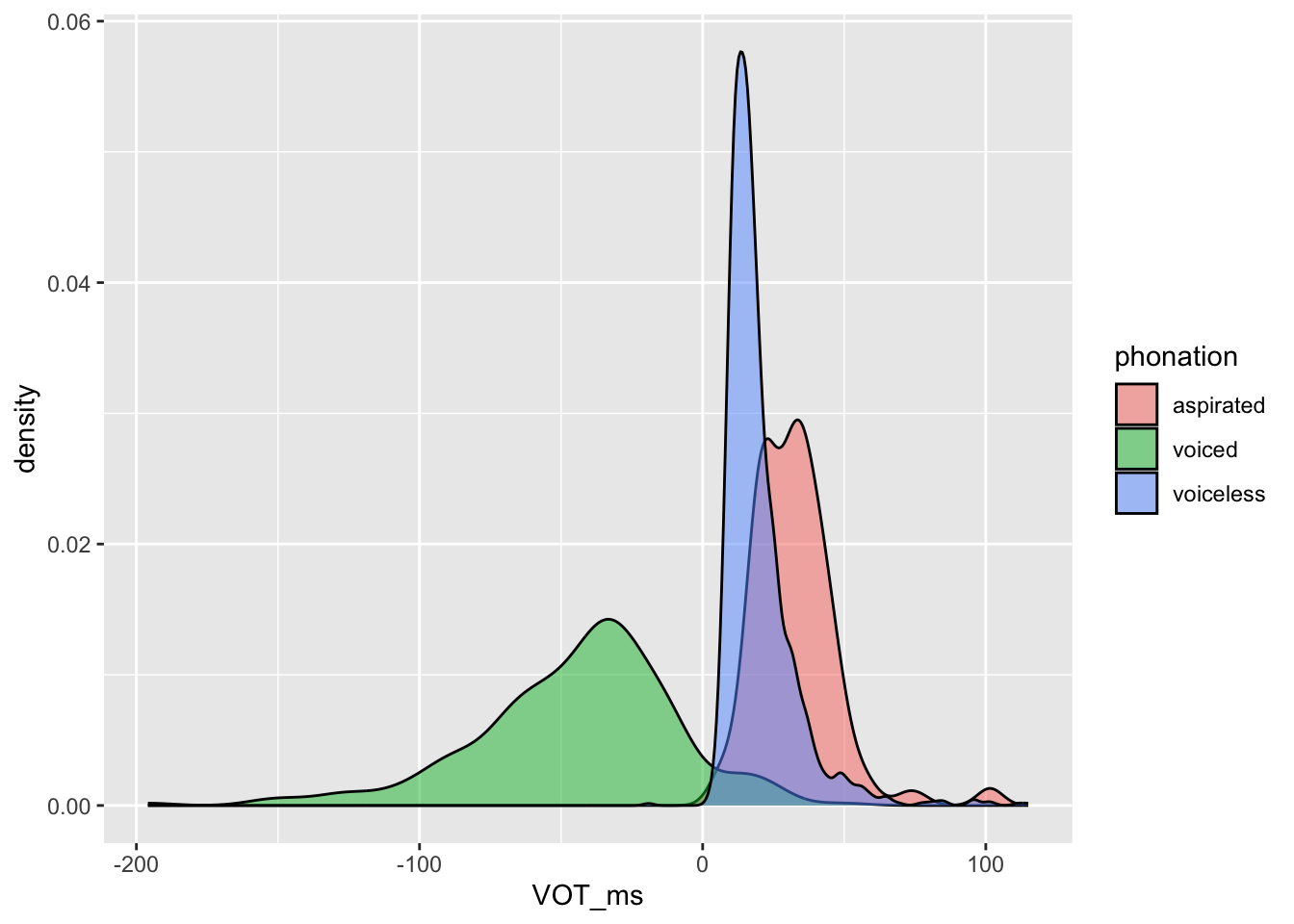
WarningExercise 1
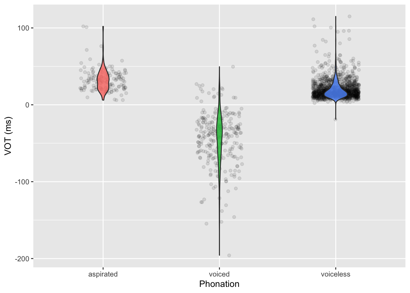
Recreate the following plot.
28.2 Treatment contrasts with three levels
Let’s proceed with modelling VOT. We will assume that VOT values follow a Gaussian distribution: as with reaction times, this is just a pedagogical step for you to get familiar with fitting models with categorical predictors, but other distribution families might be more appropriate. While for reaction times there are some recommended distributions (which you will learn about in Chapter 31), there are really no recommendations for VOT, so a Gaussian distribution will have to do for now.
Before fitting the model, it is important to go through the model’s mathematical formula and to pay particular attention to how phonation type is coded using treatment contrasts. The phonation predictor has three levels: aspirated, voiced and voiceless. The order of the levels follows the alphabetical order. You will remember from Chapter 27 that the mean of the first level of a categorical predictor ends up being the intercept of the model while the difference of the second level relative to the first is the slope. With a third level, the model estimates another “slope”, which is the difference between the third level and the first. With treatment contrasts, the second and higher levels of a categorical predictor are compared (or contrasted) with the first level. With the default alphabetical order, this means that the intercept of the model will tell us the mean VOT of aspirated stops, and the mean of voiced and voiceless stops will be compared to that of aspirated stops.
An other important aspect of treatment coding of categorical predictors that we haven’t discussed is the number of indicator variables needed: the number of indicator variables is always the number of the levels of the predictor minus one (\(N - 1\), where \(N\) is the number of levels). It follows that a predictor with three levels needs two indicator variables (\(N = 3\), \(3 - 1 = 2\)). This is illustrated in Table 28.1. For each observation, \(ph_\text{VD}\) indicates if the observation is from a voiced stop (1) or not (0), and \(ph_\text{VL}\) indicates if the observation is from a voiceless (unaspirated) stop (1) or not (0). Of course, if the observation if from an aspirated stop, that is neither a voiced nor a voiceless (unaspirated) stop, so both \(ph_\text{VD}\) and \(ph_\text{VL}\) are 0.
phonation.
phonation |
\(ph_\text{VD}\) | \(ph_\text{VL}\) |
|---|---|---|
phonation = aspirated |
0 | 0 |
phonation = voiced |
1 | 0 |
phonation = voiceless |
0 | 1 |
Now that we know how phonation is coded, we can look at the model formula.
\[ \begin{aligned} \text{VOT}_i & \sim Gaussian(\mu_i, \sigma)\\ \mu_i & = \beta_0 + \beta_1 \cdot ph_{\text{VD}[i]} + \beta_2 \cdot ph_{\text{VL}[i]}\\ \end{aligned} \]
The formula states that each observation of VOT come from a Gaussian distribution with a mean and standard deviation and that the mean depends on the value of the indicator variables \(ph_\text{VD}\) and \(ph_\text{VL}\): that is what the subscript \(i\) is for.
The code below fits a Gaussian regression model, with VOT (in milliseconds) as the outcome variable and phonation type as the (categorical) predictor. Phonation type (phonation) is coded with treatment contrasts. Before fitting the model, answer the question in Quiz 1 below.
library(brms)

vot_bm <- brm(
  VOT_ms ~ phonation,
  family = gaussian,
  data = eu_vot,
  seed = 6725,
  file = "cache/ch-regression-more-vot_bm"
)When you run the model you will see this message: Warning: Rows containing NAs were excluded from the model.. This is really nothing to worry about: it just warns you that rows that have NAs were dropped before fitting the model. Of course, you could also drop them yourself in the data and feed the filtered data to the model. This is probably a better practice because it gives you the opportunity to explicitly find out which rows have NAs (and why).
Carefully look through the Regression Coefficients of the model and make sure you understand what each row corresponds to. It should be clear by now that while the first coefficient, the “intercept”, is the mean VOT with aspirated stops, the second and third coefficients are the difference between the mean VOT of aspirated stops and the mean VOT of voiced and voiceless stops respectively. This falls out of the formulae you worked out in Exercise 3.
28.3 Posterior predictions
We can obtain the posterior predictions for the VOT of voiced and voiceless stops as we did in Section 27.4. If you have completed Exercise 3 above, the following code should have no surprises.
vot_bm_draws <- as_draws_df(vot_bm) |>
  mutate(
    aspirated = b_Intercept,
    voiced = b_Intercept + b_phonationvoiced,
    voiceless = b_Intercept + b_phonationvoiceless
  )
Let’s also pivot the draws to a longer format with pivot_longer(). Ignore the warning about dropping the draws_df class.
vot_bm_long <- vot_bm_draws |>
  select(aspirated:voiceless) |>
  pivot_longer(everything(), names_to = "phonation", values_to = "pred")
Warning: Dropping 'draws_df' class as required metadata was removed.vot_bm_longThis time I will show you how to use the long draws tibble to create a summary table. This is what the following code does: the only new bit is the paste(..., collapse = ", ") part. This is needed because quantile2() returns a vector with two elements (one with the lower limit and one with the upper limit of the CrI) but we want to collapse that into a single string, with the two limits separated by a comma and space. The resulting string is wrapped between square brackets, a typical format for reporting CrIs.
vot_bm_tab <- vot_bm_long |>
  group_by(phonation) |>
  summarise(
    mean = mean(pred), sd = sd(pred),
    `99%` = paste0("[", paste(quantile2(pred, c(0.005, 0.995)) |> round(), collapse = ", "), "]"),
    `60%` = paste0("[", paste(quantile2(pred, c(0.2, 0.8)) |> round(), collapse = ", "), "]")
  )

vot_bm_tab
The function kable() from the knitr package provides us with a convenient way to output the table in vot_bm_tab as a nicely formatted table in a rendered Quarto file. Table 28.2 is indeed the output of R code using knitr::kable(). Unfold the code to see it (click on the little triangle to the left of Code below). Check the documentation of kable() to learn about its arguments.
Code
vot_bm_tab |>
  knitr::kable(
    col.names = c("", "Mean", "SD", "99% CrI", "60% CrI"),
    digits = 1, align = c("rcccc")
)| Mean | SD | 99% CrI | 60% CrI | |
|---|---|---|---|---|
| aspirated | 32.6 | 1.5 | [29, 37] | [31, 34] |
| voiced | -44.4 | 1.1 | [-47, -42] | [-45, -43] |
| voiceless | 19.8 | 0.5 | [19, 21] | [19, 20] |
In Table 28.2, I reported the posterior mean, SD and 99% and 60% CrIs of the posterior distributions of the predicted VOT of aspirated, voiced, and voiceless stops. Why 99% and 60%? There is nothing special with 95% CrIs and as mentioned in previous chapters you should report multiple levels. I admit that in this case, as in the models from previous chapters reporting more than one CrI is overkill, because our posteriors are so certain. So take this as just an example of how you could report results in a table. Probably, a 99% CrI would have sufficed.
28.4 Reporting
The following paragraph shows you how you could write up the model and results in a paper.
We fitted a Bayesian regression model to Voice Onset Time (VOT) of Mixean Basque stops. We used a Gaussian distribution for the outcome and phonation (aspirated, voiced, voiceless) as the only predictor. Phonation was coded using the default treatment coding.
According to the model, the mean VOT of aspirated stops is between 29 and 37 ms, of voiced stops is between -47 and -42 ms, of voiceless stops is between 19 and 21 ms, at 99% probability. Table 28.2 reports mean, SD, 99% and 60% CrIs. When comparing voiced and voiceless stops to aspirated stops, at 99% confidence, the VOT of voiced stops is 72-82 ms shorter than that of aspirated stops (mean = -77, SD = 1.86), while the VOT of voiceless stops is 9-17 ms shorter than that of aspirated stops (mean = -13, SD = 1.58).
You might find that certain authors use \(\beta\) instead of “mean” for the posterior mean reported between parentheses: for example, (\(\beta\) = 33, SD = 1.5). The \(\beta\) stands for \(\hat{\beta}\), which is a notation to indicate that the \(\beta\) is estimated (that’s what the little hat on top of the letter signifies). This practice is probably more common in the frequentist approach than the Bayesian approach to inference. I find it more straightforward to say “mean” since that is what the estimand is: the mean of the posterior distribution of the coefficient. Similarly, some might use “SE” for standard error instead of SD. As long as one is consistent, it doesn’t matter much since there are indeed different traditions (and even different fields within linguistics might prefer different ways of reporting).
Note that readers not used to Bayesian statistics might find the choice of CrI levels questionable or at least surprising. As said many times, there is nothing special about 95% CrI: it is a misguided historical accident from frequentist approaches to default to 95%. The next chapter is dedicated precisely to frequentist statistics and how this approach is misused in research. Most of the current research in linguistics is conducted using problematic frequentist methods, so the only thing you can do is learn where the problems lie and do your best to avoid them in your own research.