set.seed(2953)
# Vowel duration before voiceless consonants
vdur_vls <- rnorm(15, mean = 80, sd = 10)
vdur_voi <- rnorm(15, mean = 90, sd = 10)29 Frequentist statistics, the Null Ritual and p-values
![]()
![]()
In Chapter 20, you were introduced to the Bayesian approach to inference, and we only briefly mentioned frequentist statistics. It is very likely that you had heard of p-values before, especially when reading research literature. You will have also heard of “statistical significance”, which is based on the p-value obtained in a statistical test performed on data. This section will explain what p-values are, how they are often misinterpreted and misused (Cassidy et al. 2019; Gigerenzer 2004), and how the “Null Ritual”, a degenerate form of statistics derived from different frequentist frameworks (yes, you can do frequentist statistics in different ways!) has become the standard in research, despite not being a coherent way of doing frequentist statistics (Gigerenzer, Krauss, and Vitouch 2004).
29.1 Frequentist statistics, feuds and eugenics: a brief history
A lot of current research is carried out with frequentist methods. This is a historical accident, based on both an initial misunderstanding of Bayesian statistics (which is, by the way, older than frequentist statistics) and the fact that frequentist maths was much easier to deal with (and personal computers did not exist at the time). Bayesian statistics, rooted in Thomas Bayes‘s (1701-1771) work on updating probabilities with new evidence based on a specific interpretation of Bayes’ Theorem, remained largely dormant until the 20th century due to computational difficulties and philosophical debates. It gained widespread traction in the 1990s with advances in computational methods, especially the development of Markov Chain Monte Carlo ( Chapter 25). However, modern frequentist statistics is attributed to three statisticians whose lives span several decades before the time Bayesianism found a place in statistical debates: Ronald Fisher (1890-1926), Jerzy Neyman (1894-1981) and Egon Pearson (1895-1980, the son of another statistician, Karl Pearson 1857-1936).
The history of frequentist statistics is a tale of heated debates, feuds and the now discredited field of eugenics (a colonial movement with the aim of improving the genetic “quality” of human populations). Francis Galton (1822-1911) is considered the originator of eugenics: this is the same Galton who came up with the idea of “regression toward mediocrity” which gives the name to regression models (see Spotlight box in Chapter 23). Karl Pearson was deeply influenced by Galton and saw statistics as a tool for improving racial fitness. Pearson’s Biometric School in Britain was explicitly tied to eugenics research. Ronald Fisher was another British statistician who strongly believed in eugenics and racial differences. While both K. Pearson and Fisher were proponents of eugenics, they differed in their understanding of statistics. Fisher criticised K. Pearson’s approach as too mechanic and simplistic (thus earning the elder statistician’s lasting disapproval). Fisher came up with the concept of statistical significance and devised the famous p-value as a way to quantify statistical significance based on data, against a hypothesis (to be nullified) of how the researcher thought the data were produced.
Fisher’s contemporaries Jerzy Neyman and Egon Pearson (the son of K. Pearson), who both rejected eugenics, found Fisher’s critiques to K. Pearson’s (the father) approach well-founded, but they themselves thought Fisher’s significance testing fell short. While Fisher’s significance testing was based on quantifying significance in light of a single hypothesis, Neyman and E. Pearson (the son) argued that one should contrast two opposing hypotheses and control for error rates in rejecting one and accepting the other. They thus introduced the idea of “significance level”, a threshold which determined if one accepted a result as statistically significant or not. In sum, while Fisher’s approach was focused on estimating the degree of statistical significance, Neyman and Pearson’s approach was more interested in decision-making under uncertainty. “Fisherian frequentism” and “Neyman–Pearson frequentism”, as they later became to be known, are incompatible approaches, despite both being based on the same statistical concept of the p-value, because they entail two very different interpretations of statistical significance (and the objective of research more generally).
29.2 Null Hypothesis Significance Testing
Moving forward in time to the last three decades, the commonly accepted approach to frequentist inference is the so-called Null Hypothesis Significance Testing, or NHST. As practised by researchers, the NHST approach is an incoherent mix of Fisherian and Neyman–Pearson frequentism (Perezgonzalez 2015). The main tenet of the NHST is that you set a null hypothesis and you try to reject it (as Fisher expected statistical significance to be used). A null hypothesis is, in practice, always a nil hypothesis: in other words, it is the hypothesis that there is no difference between two estimands (these usually being means of two or more groups of interest). This aspect is a great departure from both Fisherian and Neyman–Pearson frequentism, since neither says anything about the null hypothesis having to necessarily be a nil hypothesis. Then, using a variety of numerical techniques, one obtains a p-value, i.e. a frequentist probability. The p-value is used for inference: if the p-value is smaller than a threshold (Neyman–Pearson’s significance level), you can reject the nil hypothesis; if the p-value is equal to or greater than the threshold, you cannot reject the null hypothesis.
The following section explains p-values within the NHST approach, since that is the approach researchers adopt (knowingly or less knowingly) when using p-values. Note however that the NHST approach has been heavily criticised by frequentist and Bayesian statisticians alike and has resulted in the proposal of alternative, stricter, versions of NHST, like the frequentist Statistical Inference as Severe Testing (SIST, Mayo 2018; for a critique see Gelman et al. 2019). The inconsistent nature of NHST has led to the elaboration of the concept and label “Null Ritual” (Gigerenzer 2004, 2018; Gigerenzer, Krauss, and Vitouch 2004) and the slogan-titled paper The difference between “significant” and “not significant” is not itself statistically significant (Gelman and Stern 2006). p-values are very commonly mistaken for Bayesian probabilities (Cassidy et al. 2019) and this results in various misinterpretations of reported results. Section 29.4 explains the main issues with the Null Ritual and invites you to always think critically when reading results and discussions in published research.
29.3 The p-value
To illustrate p-values, we will compare simulated durations of vowels when followed by voiceless consonants vs voiced consonants. It is a well-known phenomenon that vowels followed by voiced consonants tend to be longer than vowels followed by voiceless ones (see review in Coretta 2019). Let’s simulate some vowel duration observations: we do so with the rnorm() function, which takes three arguments: the number of observations to sample and the mean and standard deviation of the Gaussian distribution to sample observations from. We use a \(Gaussian(80, 10)\) for durations before voiceless consonants, and a \(Gaussian(90, 10)\) for durations before voiced consonants. In other word, there is a difference of 10 milliseconds between the two means. Since the rnorm() function randomly samples from the given distribution, we have set a “seed” so that the code will return the same numbers every time it is run, for reproducibility.
Normally, you don’t know what the underlying means are, we do here because we set them. So let’s get the sample mean of vowel duration in the two conditions, and take the difference.
mean_vls <- mean(vdur_vls)
mean_voi <- mean(vdur_voi)

diff <- mean_voi - mean_vls
diff
[1] 7.43991The difference in the sample means is about 7.4. Now, a NHST researcher would define the following two hypotheses:
\(H_0\): the difference between means is 0.
\(H1\): the difference between means is not 0.
\(H_0\) simply states that there is no difference between the mean of vowel duration when followed by voiced or voiceless consonants. This is the “null” hypothesis. \(H_1\), called the “alternative” hypothesis, states that the difference between means is different from exactly 0. We could have decided to go with “greater than 0”, rather than just “not 0”, because we know about the trend of longer vowels before voiced consonants, so the difference should be positive. But this is not how NHST is usually set up: it is always assumed that the \(H_1\) is “the difference between means is not 0”.
Here is where things get tricky: if \(H_0\) is correct, then we should observe a difference as close to 0 as possible. Why not exactly 0? Because it is impossible for two samples (even if they come from exactly the same distribution) to have exactly the same mean for the difference to be 0. But how do we define “as close as possible”? The frequentist solution is to define a probability distribution of the difference between means centred around 0. This means that 0 has the highest probability, but that negative and positive differences around 0 are also possible.
William Sealy Gosset (1876-1937), a statistician, chemist and brewer who worked for Guinness the brewery, proposed the t-distribution for this purpose. Gosset, though employed at Guinness, was sent to University College London in 1906–1907 to study statistics under Karl Pearson (the father), who at the time was the leading authority in mathematical statistics. Guinness allowed this because Gosset needed advanced statistical tools to handle small experimental data sets in brewing and agriculture. K. Pearson’s Biometrika journal became the outlet where Gosset published his famous 1908 paper “The probable error of a mean” (Student 1908). K. Pearson encouraged Gosset to publish it, though Guinness insisted that he use a pseudonym to protect trade secrets, so Gosset published under the pseudonym “Student”. Because of this, the t-distribution is also called the Student-t distribution. Gosset argued that the t-distribution was an appropriate probability distribution for differences between means, especially with small sample sizes.
The t-distribution is similar to a Gaussian distribution, but the probability on either side of the mean declines more gently than with the Gaussian. As the Gaussian, the t-distribution has a mean and a standard deviation. It has an extra parameter: the degrees of freedom, or \(df\). The \(df\) affect how quickly the probability declines moving away from zero: the higher the \(df\) the more quickly the probability gets lower. This is illustrated in Figure 29.1. The figure shows four different t-distributions: what they all have in common is that the mean is 0 and the standard deviation is 1. These are called “standard” t-distributions. Where they differ is in their degrees of freedom. When the degrees of freedom are infinite (Inf), the t-distribution is equivalent to a Gaussian distribution.
Code
# Degrees of freedom to compare
dfs <- c(1, 2, 5, Inf)

# Create data
data <- tibble(df = dfs) |>
  mutate(data = map(df, ~ {
    tibble(
      x = seq(-4, 4, length.out = 500),
      y = if (is.infinite(.x)) dnorm(seq(-4, 4, length.out = 500))
          else dt(seq(-4, 4, length.out = 500), df = .x)
    )
  })) |>
  unnest(data)

# Plot
ggplot(data, aes(x = x, y = y, color = as.character(df))) +
  geom_line(linewidth = 1) +
  labs(
    title = "t-Distributions",
    x = "t-statistic", y = "Density",
    color = "DFs"
  ) +
  scale_color_brewer(palette = "Set1")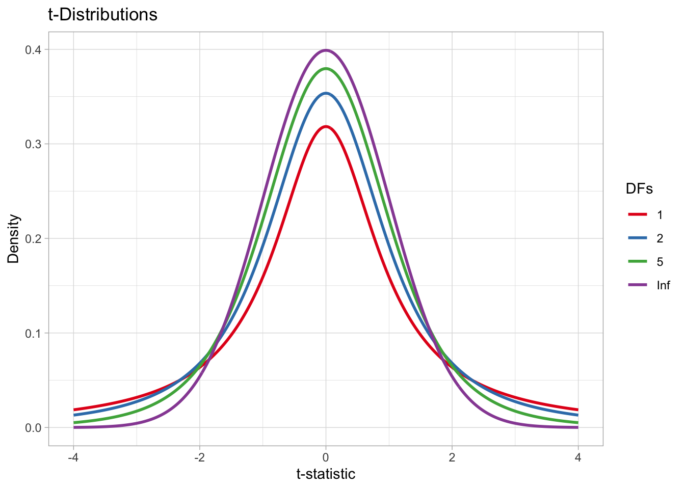
Why mean 0 and standard deviation 1? Because we can standardise the difference between the two means and always use the same standard t-distribution, so that the scale of the difference doesn’t matter: we could be comparing milliseconds, or Hertz, or kilometres. To standardise the difference between two means, we calculate the t-statistic. The t-statistic is a standardised difference. Here’s the formula:
\[ t = \frac{\bar{x}_1 - \bar{x}_2}{\sqrt{\frac{s_1^2}{n_1} + \frac{s_2^2}{n_2}}} \]
\(t\) is the t-statistic.
\(\bar{x}_1\) and \(\bar{x}_2\) are the sample means of the first and second group (the order doesn’t really matter).
\(s^2_1\) and \(s^2_2\) are the variance of the first and second group. The variance is simply the square of the standard deviation (expressed with \(s\) here).
\(n_1\) and \(n_2\) are the number of observations for the first and second group (sample size).
We have the means of vowel duration before voiced and voiceless consonants and we know the sample size (15 observations per group), so we just need to calculate the variance.
var_vls <- sd(vdur_vls)^2 # also var(vdur_vls)
var_voi <- sd(vdur_voi)^2 # also var(vdur_voi)

tstat <- (mean_voi - mean_vls) / sqrt((var_voi / 15) + (var_vls / 15))

tstat
[1] 2.437442So the t-statistic for our calculated difference is 2.4374424. Gosset introduced the t-statistics as a tool for quantile interval estimation and for comparing means, but hypothesis testing wouldn’t be “invented” until Fisher’s work on the p-value one or two decades later. Fisher took Gosset’s t-statistic and embedded it into his broader significance testing framework. Fisher popularized the use of the t-distribution for calculating p-values: the probability, under the null hypothesis, of obtaining a t-statistic as extreme or more extreme than the observed value. This re-framing changed the purpose of Gosset’s work from estimation to a frequentist test of significance.
Now, after having obtained the t-statistic, the NHST researcher would ask: what is the probability of finding a t-statistic (and the difference in means it represents) this large or larger, assuming that the t-statistic (and the difference) is 0. This probability is Fisher’s p-value. You should note two things:
First, the part about the real difference being 0. This is \(H_0\) from above, our null hypothesis that the difference is 0. For a p-value to work, we must assume that \(H_0\) is always true. Otherwise, the frequentist machinery does not work.
Another important aspect is the “difference this large or larger”: due to how probability density functions work, we cannot obtain the probability of a specific value, but only the probability of an interval of values (Chapter 19). The NHST story goes that, if \(H_0\) is true, you should not get very large differences, let alone larger differences than the one found.
The next step is thus to obtain the probability of \(t \geq\) 2.4374424 (t being equal to or greater than 2.4374424), given a standard t-distribution. Before we can do this we need to pick the degrees of freedom of the distribution, because of course these affect the probability. The degrees of freedom are calculated based on the data with the following, admittedly complex, formula:
\[ \nu = \frac{\left( \frac{s_1^2}{n_1} + \frac{s_2^2}{n_2} \right)^2}{\frac{\left( \frac{s_1^2}{n_1} \right)^2}{n_1 - 1} + \frac{\left( \frac{s_2^2}{n_2} \right)^2}{n_2 - 1}} \]
Code
df <- ( (var_voi/15 + var_vls/15)^2 ) /
      ( ((var_voi/15)^2 / (15 - 1)) + ((var_vls/15)^2 / (15 - 1)) )
The degrees of freedom for our data are approximately 28. Figure 29.2 shows a t-distribution with those degrees of freedom and a dashed line where our t-statistic falls. Now, since we set \(H_1\) to be “the difference is not 0”, we are including both positive and negative differences between the means. The sign of the t-statistic reflects the sign of the difference: positive t means a positive difference, while negative t indicates a negative difference between the two means. Since \(H_1\) is non-directional (it does not specify whether the difference is positive or negative), the p-value must account for extreme values of the t-statistic in both directions. This is called a two-tailed t-test: the p-value is the probability of observing a t-statistic at least as extreme as the one obtained, in either tail of the t-distribution.
Code
# Create data
data <- tibble(df = df) |>
  mutate(data = map(df, ~ {
    tibble(
      x = seq(-4, 4, length.out = 500),
      y = if (is.infinite(.x)) dnorm(seq(-4, 4, length.out = 500))
          else dt(seq(-4, 4, length.out = 500), df = .x)
    )
  })) |>
  unnest(data)

# Plot
ggplot(data, aes(x = x, y = y)) +
  geom_line(linewidth = 1) +
  geom_vline(xintercept = tstat, linetype = "dashed") +
  geom_vline(xintercept = -tstat, linetype = "dotted") +
  geom_area(
    data = subset(data, x >= tstat),
    aes(x = x, y = y),
    fill = "purple", alpha = 0.3
  ) +
  geom_area(
    data = subset(data, x <= -tstat),
    aes(x = x, y = y),
    fill = "purple", alpha = 0.3
  ) +
  annotate(
    "text", x = 3, y = 0.05, label = "t-statistic"
  ) +
  labs(
    title = glue::glue("Standard t-Distribution with df = {round(df)}"),
    x = "t-statistic", y = "Density",
    caption = "The sum of the shaded areas is the p-value."
  )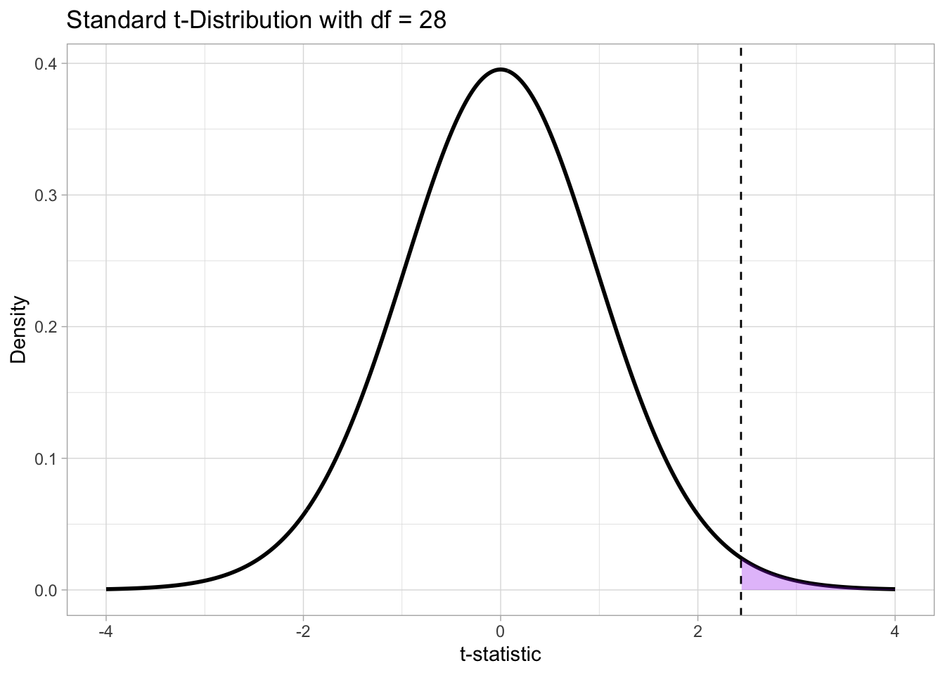
In Figure 29.2, the dotted line to the left of the distribution marks the t-statistic but with negative sign. The shaded purple area on both tails of the distribution marks the area under the density curve with t values as extreme or more extreme than the obtained t-statistic. The size of this area is the probability that we get a t value as extreme or more extreme than the obtained t-statistic, given that \(H_0\) is true. This probability is the p-value! The part “given that \(H_0\) is true” shows that the p-value is a conditional probability, conditional on \(H_0\) being true: we could write this as \(p = P(d | H_0)\), where the vertical bar \(|\) indicates that the probability of the t-statistic is conditional on \(H_0\) and \(d\) stands for “data”, or more precisely for “data as extreme or more extreme than the one observed”. You have already encountered conditional probabilities in Chapter 20, in Bayes’ Theorem.
You can get the p-value in R using the pt() function. You need the t-value and the degrees of freedom. These are saved in tstat and df from previous code. We also need to set another argument, lower.tail: this argument, when set to TRUE, states that we want the probability of getting a t value that is equal to or less than the specified t value, but we want the probability of getting a t value that is equal to or greater than the specified t value, since the t-value is positive, so we set lower.tail to FALSE. Since this is a two-tailed t-test, we also need the probability for the negative tail. Since the distribution is symmetric around 0, the upper and lower-tail probabilities given a t-statistic are the same, so we can simply multiply the upper-tail probability by 2.
# pt() times 2 to get the two-tailed prob
pvalue <- pt(tstat, df, lower.tail = FALSE) * 2
pvalue
[1] 0.02150441In other words, assuming \(H_0\) is true and there is not difference between the two groups of vowel duration, the probability of obtaining a t-statistic as extreme or more extreme than \(\pm\) 2.44 is approximately 0.02. In other words, there is approximately a 2% probability that the difference between durations of vowels followed by voiced or voiceless consonants is \(\pm\) 7 ms or larger. Of course, we want the p-value to be as small as possible: if \(H_0\) is true and the true difference is 0, finding a large difference should be very unlikely (think about the t-distribution: values away from 0 are less likely than 0 and values closer to 0). This was the original formulation of Fisher’s statistical testing: the p value could be taken as the degree of significance. However, Neyman and Pearson argued that a threshold should be decided and that a binary decision regarding significance should be made.
How do we choose how small a p-value is small enough? Is 1% small enough? What about 0.5%? 5%?, maybe 10%? This is what the so-called \(\alpha\)-level is for (read “alpha level”, from the Greek letter \(\alpha\)). We will get back to the issue of setting an \(\alpha\)-level in the next section, but for now know that in social research it has become standard to set it to 0.05. In other words, if the p-value is lower than \(\alpha = 0.05\) then we take the p-value to be small enough, otherwise we don’t. When the p-value is smaller than 0.05, we say we found a statistically significant difference, when it is equal to or greater than 0.05, we say we found a statistically non-significant difference. When we find a statistical significant difference, the NHST story goes, we say that we reject the null hypothesis \(H_0\). In our simulated example of vowel duration, the p-value is smaller than 0.05, so we say the mean vowel durations before voiced vs voiceless consonants are (statistically) significantly different from each other.
29.4 The Null Ritual
Gigerenzer (2004) calls the way researchers perform NHST the “null ritual”. He defines the null ritual as the following procedure (Gigerenzer 2004, 588):
Set up a statistical null hypothesis of “no mean difference” or “zero correlation.” Don’t specify the predictions of your research hypothesis or of any alternative substantive hypotheses.
Use 5% as a convention for rejecting the null. If significant, accept your research hypothesis. Report the result as p < 0.05, p < 0.01, or p < 0.001 (whichever comes next to the obtained p-value).
Always perform this procedure.
Gigerenzer (2004) explains how the null ritualistic approach to frequentism, or NHST, is an inconsistent hybrid of Fisher’s statistical significance testing and Neyman–Pearson decision theory. Fisherian frequentism did not have an \(\alpha\)-level: the p-value was used as a degree of statistical significance. Neyman and Pearson rejected the idea of significance degree and argued for the use an \(\alpha\)-level, but they in no way proposed a fixed level and, quite the opposite, urged researchers to set the \(\alpha\)-level on a case-by-case basis. Moreover, Fisher’s null hypothesis didn’t have to be a nil hypothesis: you could set your null hypothesis (the hypothesis to be “nullified”) to anything it made sense, so you could have for example \(H_0: \delta = +2.5\) (where \(\delta\) “delta” is the difference between means) and the p-value would be about nullifying that hypothesis, not \(\delta = 0\).
There is another level that is relevant to Neyman–Pearson statistics that is very often glossed over: the \(\beta\)-level, also known as statistical power. Statistical power is the probability of finding a significant difference when there is a real difference. In social sciences, this is arbitrarily set to 0.8: i.e., there should be an 80% probability of finding a significance difference where there is one. Statistical power is in large part determined by the magnitude of the difference and the variance of the groups being compared. With small and very noisy differences, you need a larger sample size to reach a high statistical power. As with the \(\alpha\)-level, a researcher should set the \(\beta\)-level on a case-by-case basis. Once a statistical power level is chosen, a researcher is supposed to run a prospective power analysis (Brysbaert and Stevens 2018; Brysbaert 2020): this is a procedure that, given the chosen statistical power and hypothesised difference magnitude and variance, helps you determine a specific sample size needed to reach that statistical power. Calculating p-values without prospective power analysis is incorrect and yet has become the norm.
Furthermore, researchers consistently misinterpret p-values and frequentist inference more generally (Gigerenzer, Krauss, and Vitouch 2004; Gigerenzer 2018; Perezgonzalez 2015; Cassidy et al. 2019). There is a very common tendency to confuse the p-value for the probability that the null hypothesis \(H_0\) is true. This is incorrect because the p-value is the probability \(P(d|H_0)\): it is conditional on \(H_0\) being true and it is clearly not \(P(H_0)\). Another misinterpretation takes the p-value as the inverse of the probability that \(H_1\) is true: again, this must be false because \(P(d|H_0)\) is the probability of the “data” given \(H_0\), not the probability of \(H_0\) (in which case, assuming contrasting hypotheses, then we would indeed have \(P(H_1) = -P(H_0)\)). Finally, something dubbed “Bayesian wishful thinking” by Gigerenzer (2018), is the belief that the p-value is the probability of \(H_0\) given the data (\(P(H_0|d)\)) or worse the inverse of the probability of \(H_1\) given the data (\(P(H_1|d)\)). You might see why it is called Bayesian wishful thinking: a Bayesian posterior probability, as per Bayes’ Theorem, is precisely the probability of a hypothesis given the data: \(P(h|d)\) (Chapter 20). However, a p-value is not \(P(h|d)\) but rather \(P(d|H_0)\).
These are just the main issues and misinterpretation of the null ritual NHST and if you’d like to learn more about this, I strongly recommend you read Gigerenzer (2004) and the other papers cited in this section. Gigerenzer, Krauss, and Vitouch (2004) highlights how the null ritual can indeed hurt research and anything that comes from it. Alas, as said at the beginning of this chapter, virtually all contemporary research (especially in the social sciences and hence linguistics) adopts the null ritual for statistical inference. This means, in practice, that we should always be very sceptical of statements regarding statistical significance and or strength of evidence when reading such literature and we should instead focus more on the actual estimates of the estimands of interest.
Many students (and supervisors) worry that not learning how to run many different frequentist/null-ritualistic statistical tests and regression models could make it more difficult for you to understand previous literature, precisely because that is what most literature uses. This is in fact a unnecessary worry: all frequentist tests are just ways to obtain a p-value to test statistical significance and they tell you nothing else about the magnitude or importance of an estimate; frequentist regression models function on the same premise of using the equation of a line to estimate coefficients we’ve been discussing in the regression chapters, so that the structure of model coefficients and parameters is just the same. It is the interpretation that is different: in Bayesian regression models, you get a full posterior probability distribution for each parameter, while in frequentist regressions you only get a point-estimate (an estimate that is a single value). In other words, once you learn the basics of Bayesian regression models, you can still interpret frequentist/null-ritualistic regression models while avoiding the common pitfalls reviewed in this chapter.
29.5 Why prefer Bayesian inference?
Now that you have a better understanding of frequentist statistics and more precisely the null ritualistic version of frequentism (or NHST) as practised by researchers, here are a few practical and conceptual reasons for why Bayesian statistics might be more appropriate in most research contexts.
29.5.1 Practical reasons
Fitting frequentist models can lead to anti-conservative p-values (i.e. increased false positive rates, called Type-I error rates: there is no effect but yet you get a significant p-value). An interesting example of this for the non-technically inclined reader can be found in Dobreva (2024). Frequentist regression models fitted with
lm()/lmer()tend to be more sensitive to small sample sizes than Bayesian models (with small sample sizes, Bayesian models return estimates with greater uncertainty, which is a more conservative approach).While very simple models will return very similar estimates whether they are frequentist or Bayesian, in most cases more complex models won’t converge if run with frequentist packages like lme4, especially without adequate sample sizes. Bayesian regression models always converge, while frequentist ones don’t always do.
Frequentist regression models require as much work as Bayesian ones, although it is common practice to skip necessary steps when fitting the former, which gives the impression of it being a quicker process. Factoring out the time needed to run Markov Chain Monte Carlo chains in Bayesian regressions, in frequentist regressions you still have to perform robust perspective power analyses and post-hoc model checks.
With Bayesian models, you can reuse posterior distributions from previous work and include that knowledge as priors into your Bayesian analysis. This feature effectively speeds up the discovery process (getting to the real value estimate of interest faster). You can embed previous knowledge in Bayesian models while you can’t in frequentist ones.
29.5.2 Conceptual reasons
Frequentist regression models cannot provide evidence for a difference between groups, only evidence to reject the null (i.e. nil) hypothesis.
A frequentist Confidence Interval (CI) like a 95% CI can only tell us that, if we run the same study multiple times, 95% of the time the CI will include the real value (but we don’t know whether the CI we got in our study is one from the 5% percent of CIs that do not contain the real value). On the other hand, a 95% Bayesian Credible Interval (CrI) always tells us that the real value is within a certain range, conditional on model and data. So, frequentist models really just give you a point estimate, while Bayesian models give you a range of values and their probability.
With Bayesian regressions you can compare any hypothesis, not just null vs alternative. (Although you can use information criteria with frequentist models to compare any set of hypotheses).
Frequentist regression models are based on an imaginary set of experiments that you never actually carry out.
Bayesian regression models will converge towards the true value in the long run. Frequentist models do not.
Of course, there are merits in fitting frequentist models, for example in corporate decisions, but you’ll still have to do a lot of work. The main conceptual difference then is that frequentist and Bayesian regression models answer very different questions and as (knowledge-oriented) researchers we are generally interested in questions that the latter can answer and the former cannot.