4  R basics

4.1 Why R?

R can be used to analyse all sorts of data, from tabular data (also known as “spreadsheets”), textual data, map (GIS, Geographic Information System) data and even images.

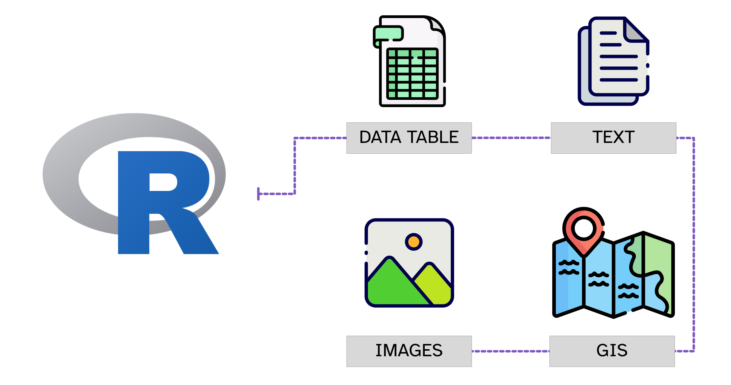
This course will focus on the analysis of tabular data, since all of the techniques relevant to this type of data also apply to the other types.

The R community is a very inclusive community and it’s easy to find help. There are several groups that promote R in minority/minoritised groups, like R-Ladies, Africa R, and Rainbow R just to mention a few.

Moreover, R is open source and free for anyone to use!

4.2 R vs RStudio

Beginners usually have trouble understanding the difference between R and RStudio. Let’s use a car analogy. What makes the car go is the engine and you can control the engine through the dashboard. You can think of R as an engine and RStudio as the dashboard.

TipR

• R is a programming language.

• We use programming languages to interact with computers.

• You run commands written in a console and the related task is executed.

TipRStudio

• RStudio is an Integrated Development Environment or IDE.

• It helps you using R more efficiently.

• It has a graphical user interface or GUI.

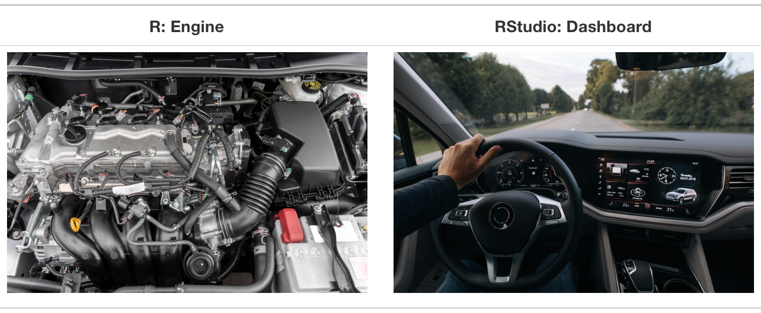
The next section will give you a tour of RStudio.

4.3 RStudio

Open RStudio on your computer and familiarise yourself with the different parts. When you open RStudio, you can see the window is divided into 3 panels:

• Blue (left): the Console.

• Green (top right): the Environment tab.

• Purple (bottom right): the Files tab.

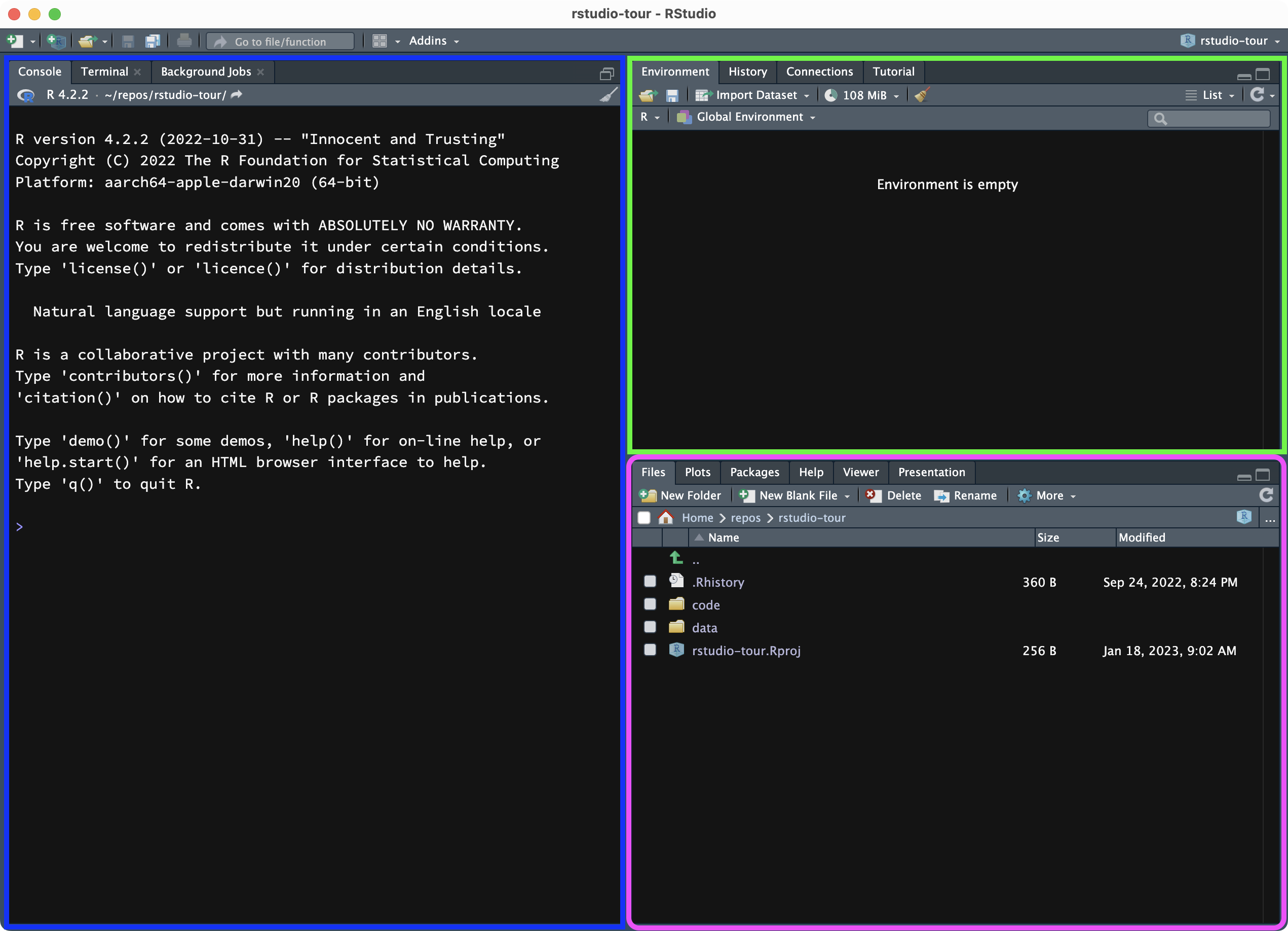
The Console is where R commands can be executed. Think of this as the interface to R. Now, try to run (execute) some R code in the console:

WarningExercise 1

• Write the following code in the Console:

  sum(3, 1, 4)

• Press ENTER/RETURN on your keyboard. This will run (i.e. execute) the code. The code sums the numbers 3, 1, and 4.

• The output of the code is shown below it, in the Console. (Never mind the [1] for now).

The Environment tab lists the objects created with R, while in the Files tab you can navigate folders on your computer to get to files and open them in the file Editor.

4.3.1 RStudio and Quarto projects

RStudio is an IDE (see above) which allows you to work efficiently with R, all in one place. Note that files and data live in folders on your computer, outside of RStudio: do not think of RStudio as an app that you can save files in. All the files that you see in the Files tab are files on your computer and you can access them from the Finder or File Explorer as you would with any other file.

In principle, you can open RStudio and then navigate to any folder or file on your computer. However, there is a more efficient way of working with RStudio: RStudio and Quarto Projects.

TipProjects

An RStudio Project is a folder on your computer that has an .Rproj file.

A Quarto Project is an RStudio Project with a _quarto.yml file.

You can create as many Quarto Projects as you wish, and I recommend to create one per project (your dissertation, a research project, a course, etc…). We will create a Quarto Project for this course (meaning, you will create a folder for the course which will be the Quarto Project). You will have to use this project/folder throughout the semester.

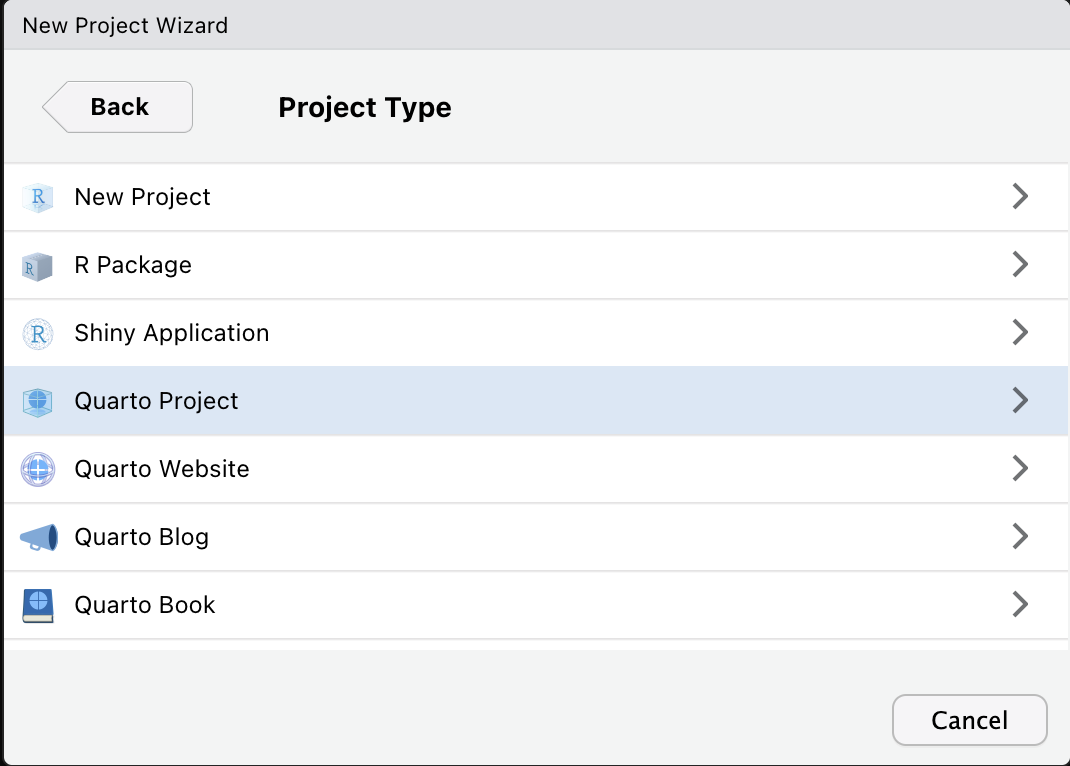
To create a new Quarto Project, click on the button that looks like a transparent light blue box with a plus, in the top-left corner of RStudio. A window like the one below will pop up.

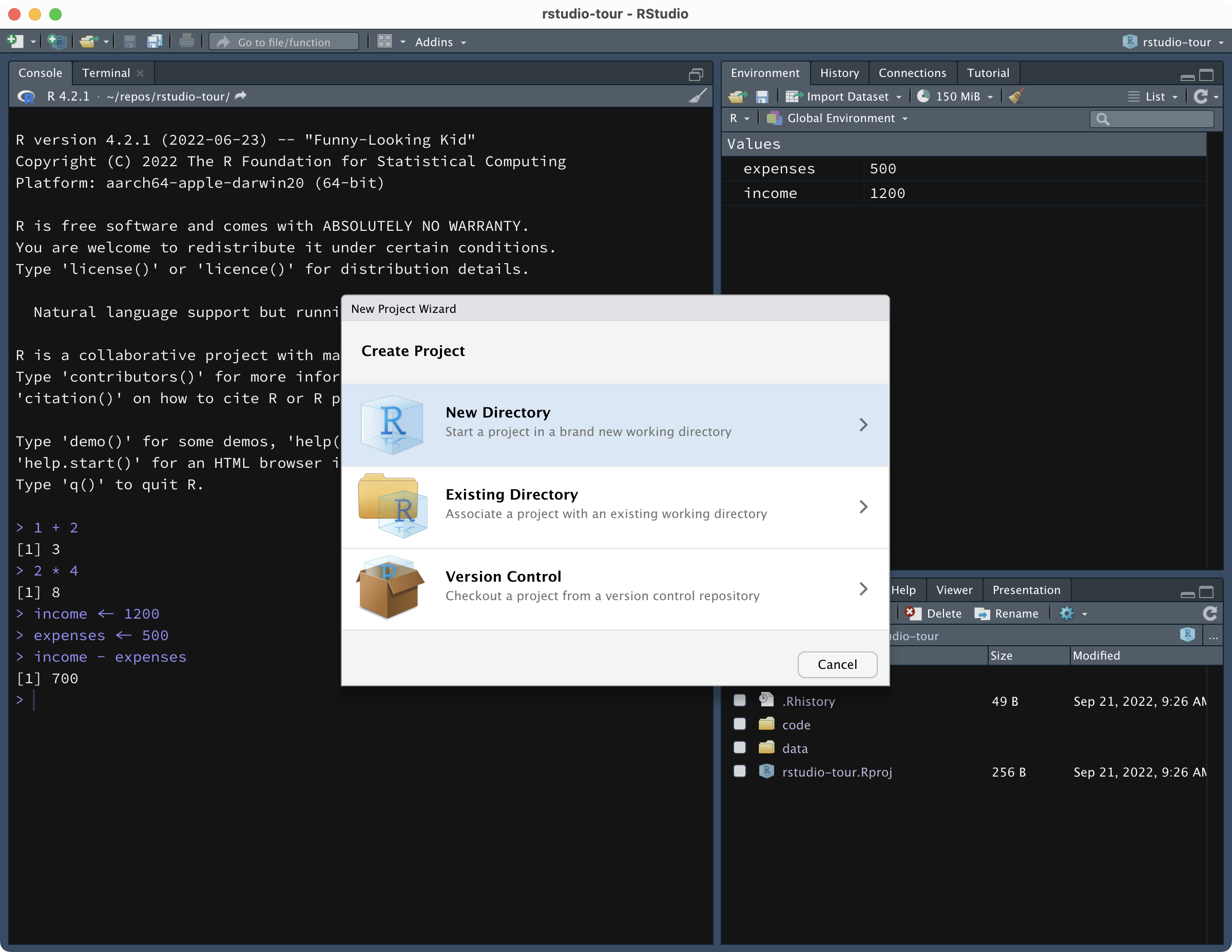
Click on New Directory then Quarto Project.

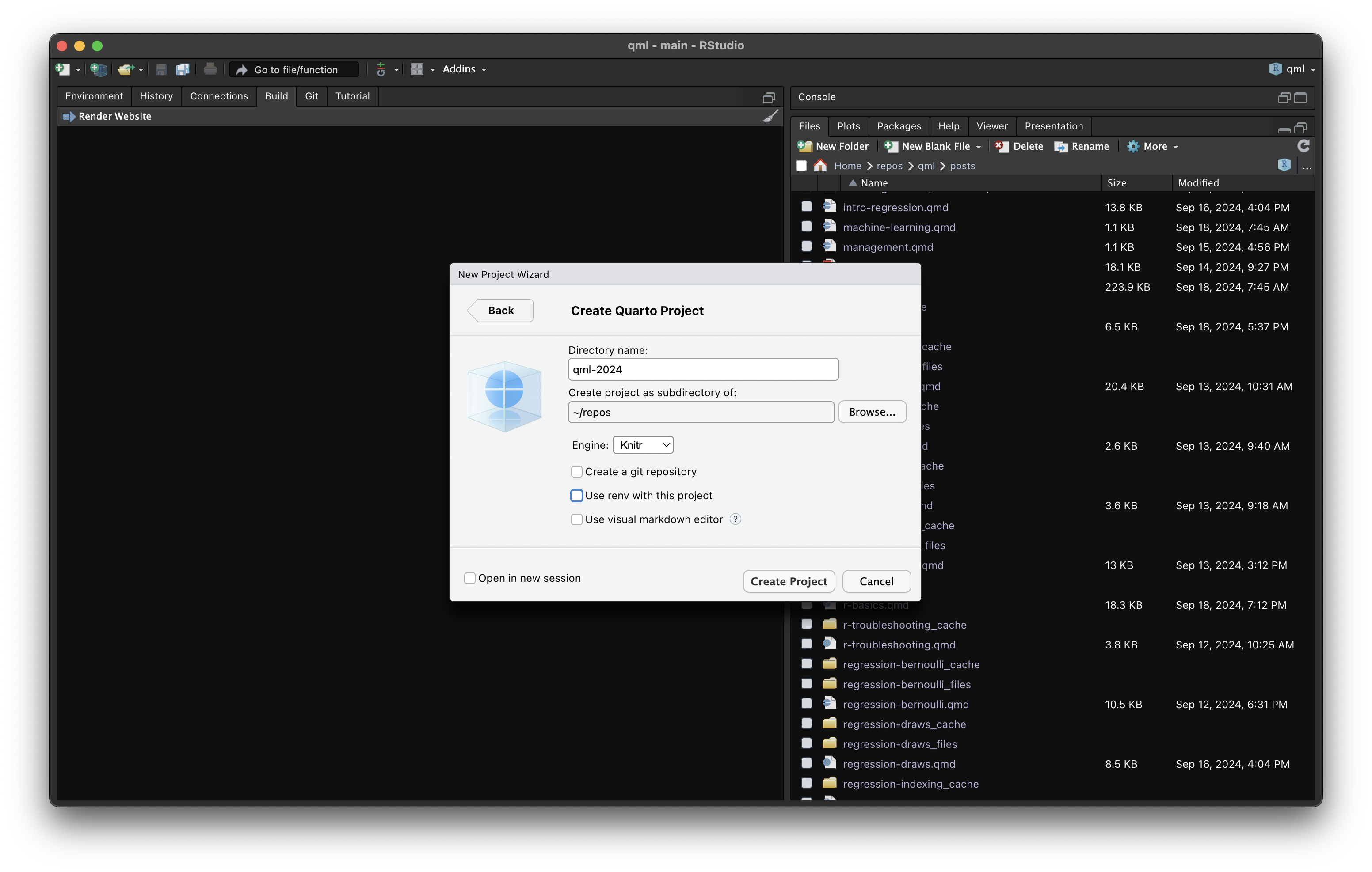
Now, this will create a new folder (aka directory) on your computer and will make that a Quarto Project (meaning, it will add a file with the .Rproj extension and a file called _quarto.yml to the folder; the name of the .Rproj file will be the name of the project/folder).

Give a name to your new project, something like the name of the course and year (e.g. qml-2025).

Then you need to specify where to create this new folder/Project. Click on Browse… and navigate to the folder you want to create the new folder/Project in. This could be your Documents folder, or the Desktop (we had issues with OneDrive in the past, so we recommend you save the project outside of OneDrive).

When done, click on Create Project. RStudio will automatically open your new project.

ImportantImportant

When working through this textbook, always make sure you are in the Quarto Project you just created for the course.

You know you are in an RStudio/Quarto Project because you can see the name of the Project in the top-right corner of RStudio, next to the light blue cube icon.

If you see Project (none) in the top-right corner, that means you are not in a Quarto Project.

An easy way to ensure that RStudio is opened from within a specific project, to open RStudio go to the project folder in File Explorer or Finder and double click on the .Rproj file. This will automatically open RStudio and set the project to that folder.

There are several ways of opening a Quarto Project:

• You can go to the Quarto Project folder in Finder or File Explorer and double click on the .Rproj file.

• You can click on File > Open Project in the RStudio menu.

• You can click on the project name in the top-right corner of RStudio, which will bring up a list of projects. Click on the desired project to open it.

WarningExercise 2

• Close RStudio.

• Now re-open RStudio by double-clicking on the .Rproj file of the project you created.

4.3.2 A few important settings

Before moving on, there are a few important settings that you need to change.

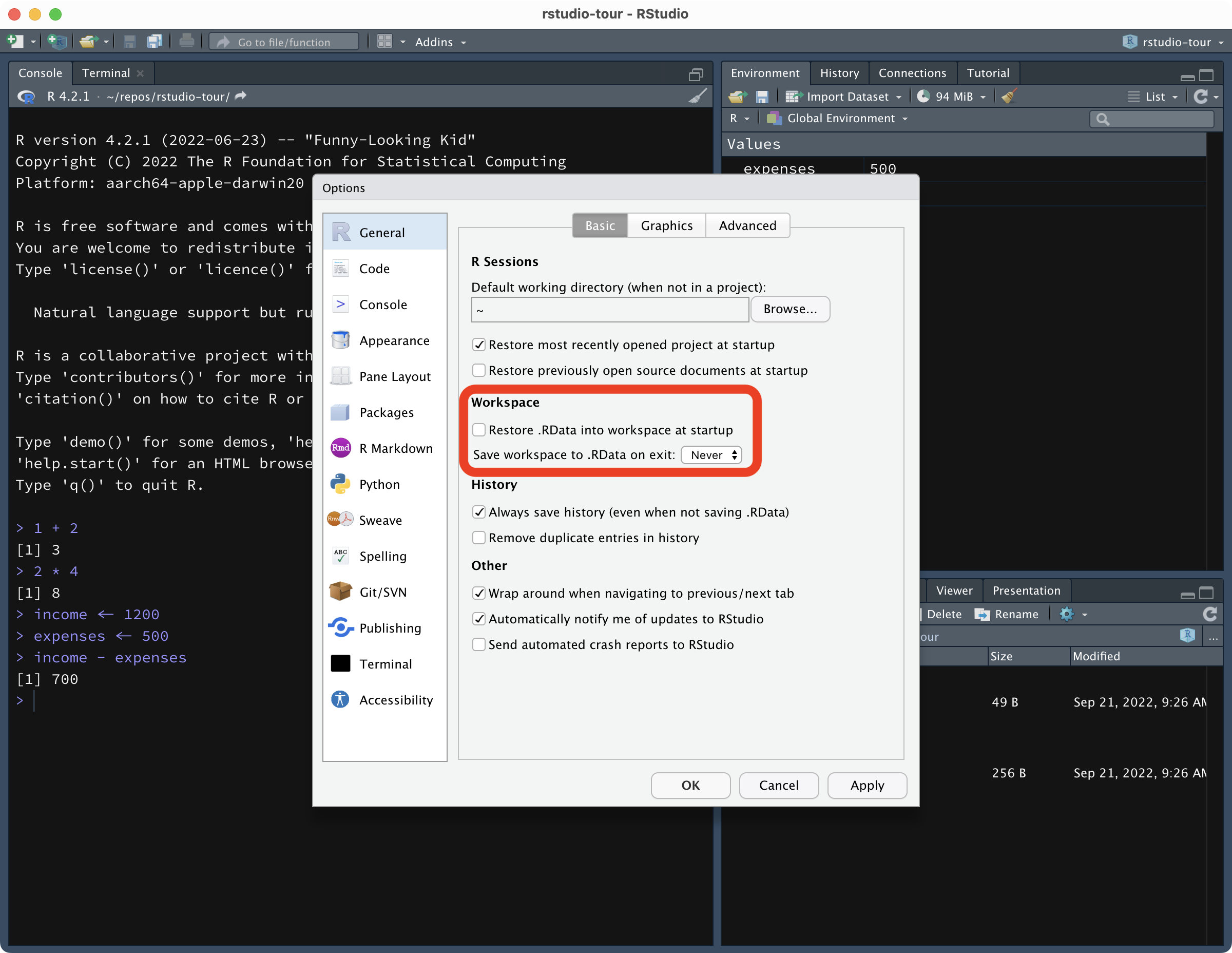
1. Open the RStudio preferences (Tools > Global options...).

2. Un-tick Restore .RData into workspace at startup.

   • This mean that every time you start RStudio you are working with a clean Environment. Not restoring the workspace ensures that the code you write is fully reproducible. When this setting is enabled, your environment is saved in a hidden file called .Rdata and loaded every time you start RStudio. This very frequently leads to errors where the wrong variables/data is read or used by the code without you noticing, so always make sure the setting is disabled.

3. Select Never in Save workspace to .RData on exit.

   • Since we are not restoring the workspace at startup, we don’t need to save it. Remember that as long as you save the code, you will not lose any of your work! You will learn how to save code from next week.

4. Click OK to confirm the changes.

NoteQuiz 1

True or false?

1. RStudio executes the code. TRUEFALSE

2. R is a programming language. TRUEFALSE

3. An IDE is necessary to run R. TRUEFALSE

4. RStudio projects are folders with an .Rproj file. TRUEFALSE

5. Quarto projects can’t be RStudio projects TRUEFALSE

6. The project name is shown in the top-right corner of RStudio. TRUEFALSE

7. I have disabled Restore .RData and Save workspace in the settings. TRUEFALSE

4.4 R basics

In this part of the tutorial you will learn the very basics of R. If you have prior experience with programming, you should find all this familiar. If not, not to worry! Make sure you understand the concepts highlighted in the green boxes and practise the related skills.

In the following sections, you should just run code directly in the R Console in RStudio, i.e. you will type code in the Console and press ENTER to run it.

In later chapters, you will learn how to save your code in a script file or in Quarto documents, so that you can keep track of which code you have run and make your work reproducible.

4.4.1 R as a calculator

Write this code 1 + 2 in the Console, then press ENTER/RETURN to run the code. Fantastic! You should see that the answer of the addition has been printed in the Console, like this:

[1] 3

(Never mind the [1] for now).

Now, try some more operations (write each of the following in the Console and press ENTER). Feel free to add your own operations to the mix!

67 - 13
2 * 4
268 / 43

You can also chain multiple operations.

6 + 4 - 1 + 2
4 * 2 + 3 * 2

NoteQuiz 2

Are the following pairs of operations equivalent?

1. 3 * 2 / 4 = 3 * (2 / 4) TRUEFALSE

2. 10 * 2 + 5 * 0.2 = (10 * 2 + 5) * 0.2 TRUEFALSE

ImportantSpotlight: Arithmetics

If you need a maths refresher, I recommend checking the following pages:

• https://www.mathsisfun.com/definitions/order-of-operations.html

• https://www.mathsisfun.com/algebra/introduction.html

4.4.2 Variables

Forget-me-not.

Most times, we want to store a certain value so that we can use it again later.

We can achieve this by creating variables.

TipVariable

A variable holds one or more values and it’s stored in the computer memory for later use.

You can create a variable by using the assignment operator <-.

Let’s assign the value 156 to the variable my_num.

my_num <- 156

Now, check the list of variables in the Environment tab of the top-right panel of RStudio. You should see the my_num variable and its value there.

Now, you can just call the variable back when you need it! Write the following in the Console and press ENTER.

my_num

[1] 156

A variable like my_num is also called a numeric vector: i.e. a vector that contains a number (hence numeric).

TipVector

A vector is an R object that contains one or more values of the same type.

A vector is a type of variable and a numeric vector is a type of vector. However, it’s fine in most cases to use the word variable to mean vector (just note that a variable can also be something else than a vector; you will learn about other R objects in later chapters).

Let’s now try some operations using variables.

income <- 1200
expenses <- 500
income - expenses

[1] 700

See? You can use operations with variables too! And you can also go all the way with variables.

savings <- income - expenses

And check the value…

savings

[1] 700

Vectors can hold more than one item or value. Just use the combine c() function to create a vector containing multiple values. The following are all numeric vectors.

one_i <- 6
# Vector with 2 values
two_i <- c(6, 8)
# Vector with 3 values
three_i <- c(6, 8, 42)

Check the list of variables in the Environment tab. You will see now that before the values of two_i and three_i you get the vector type num for numeric. (If the vector has only one value, you don’t see the type in the Enviroment list but it is still of a specific type.)

TipNumeric vector

A numeric vector is a vector that holds one or more numeric values.

Note that the following are the same:

one_i <- 6
one_i

[1] 6

one_ii <- c(6)
one_ii

[1] 6

Another important aspect of variables is that they are… variable! Meaning that once you assign a value to one variable, you can overwrite the value by assigning a new one to the same variable.

my_num <- 88
my_num <- 63
my_num

[1] 63

NoteQuiz 3

True or false?

1. A vector is a type of variable. TRUEFALSE

2. Not all variables are vectors. TRUEFALSE

3. A numeric vector can only hold numeric values. TRUEFALSE

4.4.3 Functions

R cannot function without… functions.

TipFunction

A function usually runs an operation on one or more specified arguments.

A function in R has the form function() where:

• function is the name of the function, like sum.
• () are round parentheses, inside of which you write arguments, separated by commas.

Let’s see an example:

sum(3, 5)

[1] 8

The sum() function sums the number listed as arguments. Above, the arguments are 3 and 5.

And of course arguments can be vectors!

my_nums <- c(3, 5, 7)

sum(my_nums)

[1] 15

mean(my_nums)

[1] 5

NoteQuiz 4

True or false?

1. Functions can take other functions as arguments. TRUEFALSE

2. All function arguments must be specified. TRUEFALSE

3. All functions need at least one argument. TRUEFALSE

TipHint

4c

The Sys.Date() function and other functions like it don’t take any arguments.

ImportantR Note: R vs Python

If you are familiar with Python, you will soon realise that R and Python, although they share many concepts and types of objects, can differ substantially. This is because R is a functional programming language (based on functions) while Python is an Object Oriented programming language (based on methods applied on objects).

Generally speaking, functions look like print(x) while methods look like x.print()

4.4.4 String and logical vectors

Not just numbers.

We have seen that variables can hold numeric vectors. But vectors are not restricted to being numeric. They can also store strings. A string is basically a set of characters (a word, a sentence, a full text). In R, strings have to be quoted using double quotes " ".

Change the following strings to your name and surname. Remember to use the double quotes.

name <- "Stefano"
surname <- "Coretta"

name

[1] "Stefano"

surname

[1] "Coretta"

Strings can be used as arguments in functions, like numbers can.

cat("My name is", name, surname)

My name is Stefano Coretta

Remember that you can reuse the same variable name to override the variable value.

name <- "Raj"

cat("My name is", name, surname)

My name is Raj Coretta

You can combine multiple strings into a character vector, using the combine function c() (the function works with any type of vectors, not only characters!).

TipCharacter vector

A character vector is a vector that holds one or more strings.

fruit <- c("apple", "oranges", "bananas")
fruit

[1] "apple"   "oranges" "bananas"

Check the Environment tab. Character vectors have chr before the list of values.

Another type of vector is one that contains either TRUE or FALSE. Vectors of this type are called logical vectors and they are listed as logi in the Environment tab.

TipLogical vector

A logical vector is a vector that holds one or more TRUE or FALSE values.

groceries <- c("apple", "flour", "margarine", "sugar")
in_pantry <- c(TRUE, TRUE, FALSE, TRUE)

data.frame(groceries, in_pantry)

TRUE and FALSE values must be written in all capitals and without double quotes (they are not strings!).

(We will talk about data frames, another type of object in R, in the following chapters.)

NoteQuiz 5

1. Which of the following is not a character vector.
   c(1, 2, "43") "s" c(apple) (assuming apple <- 45) c(letters)
2. Which of the following is not a logical vector.
   c(T, T, F) TRUE "FALSE" c(FALSE)

TipHint

You can use the class() function to check the type (“class”) of a vector.

class(FALSE)

[1] "logical"

class(c(1, 45))

[1] "numeric"

class(c("a", "b"))

[1] "character"

WarningExplanation

5a

• c(1, 2, "43") is a character vector because the last number "43" is a string (it’s between double quotes!). A vector cannot have a mix of types of elements: they have to be all numbers or all strings or else, but not some numbers and some strings. Numbers are special in that if you include a number in a character vector without quoting it, it is automatically converted into a string. Try the following:

char <- c("a", "b", "c")
char <- c(char, 1)
char
class(char)

• c(letters) is a character vector because letters contains the letters of the alphabet as strings (this vector comes with base R).

• c(apple) is not a character vector because the variable apple holds a number, 45!

5b

• "FALSE" is not a logical vector because FALSE has been quoted (anything that is quoted is a string!).

ImportantR Note: For-loops and if-else statements

This course does not cover programming in R in the strict sense, but if you are curious here’s a short primer on for-loops and if-else statements in R.

For-loops

fruits <- c("apples", "mangos", "durians")

for (fruit in fruits) {
  cat("I like", fruit, "\n")
}

I like apples 
I like mangos 
I like durians 

If-else

for (fruit in fruits) {
  if (grepl("n", fruit)) {
    cat(fruit, "has an 'n'", "\n")
  } else {
    cat(fruit, "does not have an 'n'", "\n")
  }
}

apples does not have an 'n' 
mangos has an 'n' 
durians has an 'n' 

For more, check the For loops section of the R4DS book and the R if else statement post from DataMentor.

4.5 Summary

You made it! You completed this chapter.

Here’s a summary of what you learned.

• R is a programming language while RStudio is an IDE.

• RStudio projects are folders with an .Rproj file (you can see the name of the project you are currently in in the top-right corner of RStudio).

• You can perform mathematical operations with +, -, *, /.

• You can store values in variables.

• A typical object to be stored in a variable is a vector: there are different type of vectors, like numeric, character and logical.

• Functions are used to perform an operation on its arguments: sum() sums its arguments, mean() calculates the mean and cat() prints the arguments.

ImportantR Note: Programming in R

If you are interested in learning about programming in R, I recommend you go through Chapters 26-28 of the R4DS book and the Advanced R book.