When working through the book, always make sure you are in a Quarto Project by checking the top-right corner of RStudio. If you see the name of the project you are fine, if you see Project (none) then you are not in the Quarto Project. Close RStudio and open the Quarto project.
Data comes in a lot of different formats, shape and sizes. However, the most common way to store data used in quantitative analysis is so-called tabular data. R is especially designed to work with such data. Tabular (aka rectangular) data is simply data in the form of a table, with columns and rows.
TipTabular data
Tabular data is data that has a form of a table: i.e. values structured in columns and rows.
Tabular data can be saved in different file formats. Different file formats have different file extensions. The comma separated values format (file extension .csv) is the best format to save data in because it is basically a plain text file, it’s quick to parse, and can be opened and edited with any software (plus, it’s not a proprietary format like .docx or .xlsx—these formats are specific to particular commercial software).
This is what a .csv file looks like when you open it in a text editor (showing only the first few lines). The file contains tabular data (data that is structured as columns and rows, like a spreadsheet).
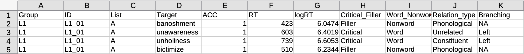
This is what the file would look like when layed out as a table.
To separate the values of each column, a .csv file uses a comma , (hence the name “comma separated values”) to separate the values in every row. The first line of the file indicates the names of the columns of the table:
This might look a bit confusing, but you will see later that, after importing this type of file, you can view it as a nice spreadsheet (as you would in Excel), like in the figure above.
Another common type of tabular data file is spreadsheets, like spreadsheets created by Microsoft Excel or Apple Numbers. These are all proprietary formats that require you to have the software that were created with if you want to modify them. Portability and openness are important aspects of conducting research, so that using open and non-proprietary file types makes your research more accessible and doesn’t privilege those who have access to specific software (remember, R is free!). Despite of this, a lot of data is shared as Excel files.
There are also variations of the comma separated values type, like tab separated values files (.tsv, which uses tab characters instead of commas) and fixed-width files (usually .txt, where columns are separated by as many white spaces as needed so that the columns align).
9.1.1 Non-tabular data
Of course, R can import also data that is not tabular, like map data and complex hierarchical data, including XML, HTML and json data. We will not cover these types of data, but you can check out the resources in the Extra box.
R has a special way of saving data: .rds files. .rds files allow you to save an R object to a file on your computer, so that you can read that file back in when you need it. A common use for .rds files is to save tabular data that you have processed so that it can be readily used in many different scripts or even by other people, but .rds files can contain any type of R objects, also lists (so not only tabular data). In the following sections you will learn how to import (aka read) three types of data: .csv, Excel and .rds files.
NoteQuiz 1
Which of the following is not tabular data.
Non-tabular data can be saved to .rds files.
9.2 Get the data
The data used in this textbook come from a variety of published and unpublished linguistic studies. You can download the data files from the QML Data website according to the following instructions.
WarningHow to get the data
Download the zip archive with all the data by clicking on the following link (if this doesn’t work, right-click and choose “Save linked file” or similar): data.zip. The data is in a zip archive.
Unzip the zip file to extract the contents. (If you don’t know how to do this, search for it online for your operating system! Zip archives are a very common way of distributing data and it is important to know how to use them).
Create a folder called data/ (the slash is there just to remind you that it’s a folder, but you don’t have to include it in the name) in the Quarto project you are using for the course. You know how to do this from Chapter 7.
Move the contents of the data.zip archive into the data/ folder.
Open a Finder or File Explorer window.
Navigate to the folder where you have extracted the zip file (it will very likely be the Downloads/ folder).
Copy the contents of the zip file.
In Finder or File Explorer, navigate to the Quarto project folder, then the data/ folder, and paste the contents in there. (You can also drag and drop if you prefer.)
The rest of this chapter will assume that you have created a folder called data/ in the Quarto project folder and that the files you downloaded are in that folder. The data folder should like something like this:
I recommend that you start being very organised with your files in other projects from now on, whether it’s for a course or your dissertation or anything else. I also suggest to avoid overly nested structures (folders in folders in folders in folders…), unless strictly necessary.
Use one folder per project. The project folder will also be your RStudio/Quarto project folder. Ideally, the project folder should have all the files related to the project (one exception is PDFs of papers that form the literature background of the project: for those I recommend using bibliography managing software, like the free Zotero or JabRef).
Separate code from data. A general recommendation is to have a folder code/ or scripts/ with all the code files of the project and a folder data/ that has all the data. This makes keeping files in order easier, since everything has its natural place.
Separate raw data from derived data. Raw data is data that you have gathered that, if lost, is lost for ever. Derived data is any data that is derived from raw data and that can be derived again (for example by running a script) if it’s deleted or corrupted.
Make raw data read-only. You should assume that anything can happen to raw data, so you should treat it as “read-only”.
To summarise, these recommendations suggest to have a folder for your research project/course/else, and inside the folder two more folders: one for data and one for code. The data/ folder could further contain raw/ for raw data (data that should not be lost or changed, for example collected data or annotations) and derived/ for data that derives from the raw data, for example through automated data processing.
It might be useful to also have a separate folder called figs/ or img/ to save figures and plots. Of course which folders you will have it’s ultimately up to you and needs will vary depending on the nature and practical aspects of each study.
9.4 Read .csv files
In this section, you will learn how to read .csv files. Reading .csv files is very easy. You can use the read_csv() function from a collection of R packages known as the tidyverse. Specifically, the read_csv() function is from the readr package, one of the tidyverse packages. If you are learning R for the first time, then you won’t already have the tidyverse packages installed (you can check in the Packages tab in the bottom-right panel). Installing the tidyverse packages is easy: you just need to install the tidyverse package and that will take care of installing the most important packages in the collection (called the “core” tidyverse packages). Note that installation of the core tidyverse packages can take some time (but remember that you do this only once). If you need to install the tidyverse packages, do it now.
ImportantDid you open the Quarto project?
Before moving on, make sure that you have opened the RStudio Quarto project correctly (see warning at the beginning of the chapter).
Now that you have ensured the tidyverse packages are available, let’s read in data from Song et al. (2020). The study consists of a lexical decision task in which participants were first shown a prime, followed by a target word for which they had to indicate whether it was a real word or a nonce word. The prime word belonged to one of three possible groups, each of which refers to the morphological relation of the prime and the target word. We will get back to this data in later chapters, so for now it is sufficient if you just read the paper’s abstract to get a general idea of the research context.
The read_csv() function from the readr package only requires you to specify the file path as a string (remember, strings are quoted between " ", for example "year_data.txt"). The data to be read are in the data/ folder, in song2020/shallow.csv. On my computer, the file path of song2020/shallow.csv is /Users/ste/qdal/data/song2020/shallow.csv, but on your computer the file path will be different, of course. However, you will learn a trick below, i.e. relative paths, that allows you to specify file paths in a shortened form.
Note that while the read_csv() function does read the data in R, you must assign the output of the read_csv() function (i.e. the data we are reading) to a variable, using the assignment arrow <-, just like we were assigning values to R variables in previous chapters. And since the read_csv() is a function from the tidyverse, you first need to attach the tidyverse packages with library(tidyverse) (remember, you need to attach packages only once per session). This will attach the core tidyverse packages, including readr. Of course, you can also attach the individual packages directly: library(readr). If you use library(tidyverse) there is no need to attach individual tidyverse packages.
Open your week-02.R script. Add the following lines in the script (don’t change the file path! explanation below) and run the code (you might want to put the library() line at the top of the script, with the other packages). The read_csv() line will print information about the data and read the data into shallow.
Rows: 6500 Columns: 11
── Column specification ────────────────────────────────────────────────────────
Delimiter: ","
chr (8): Group, ID, List, Target, Critical_Filler, Word_Nonword, Relation_ty...
dbl (3): ACC, RT, logRT

ℹ Use `spec()` to retrieve the full column specification for this data.
ℹ Specify the column types or set `show_col_types = FALSE` to quiet this message.
If you look at the Environment tab, you will see shallow listed under Data. You can preview the data by clicking on the name of the data in the Environment tab. A View tab will be opened in the top-left panel of RStudio and you will see a nicely formatted table, as you would in a programme like Excel. We will dive into this data later, so just have a peek for now.
TipData frames and tibbles
In R, a data table is called a data frame.
Tibbles are special data frames created with the read functions from the tidyverse. If you are curious about the difference, check this page.
In this textbook, “data frame” and “tibble” will be used interchangeably (since we are using the read functions from the tidyverse, all resulting data frames will be tibbles).
But wait, what is that "./data/song2020/shallow.csv"? That’s a relative path. Let’s understand the concept of relative paths now.
9.4.1 Relative paths
File paths can be specified in two formats. One format is called absolute file path. An absolute file path include all folders from the top-most folder, which is normally your computer’s hard drive. For example, /Users/ste/qdal/data/song2020/shallow.csv from above is an absolute path. You know it’s an absolute path because it starts with the forward slash /. This means that there isn’t anything above Users/: it’s the top-most folder. A downside of absolute paths is that they are not portable: if I move the qdal/ folder to ste/Documents then I need to change every occurrence in my scripts to /Users/ste/Documents/qdal/data/song2020/shallow.csv. Moreover, when you share your research code (and you should!), using absolute paths means that each person that wants to run the code has to update the absolute path to reflect their own.
A solution is to use relative paths. Relative paths work by including the path only from within a specific folder. Whichever folders contain that specific folder do not matter. The specific folder is called the working directory. When you are using Quarto projects, the working directory is the project folder, i.e. the folder with the .Rproj and _quarto.yml files.
TipWorking directory
The working directory is the folder which relative paths are relative to.
When using Quarto projects, the working directory is the project folder.
Relative paths are specified by starting the path with ./. For example, if your project is called awesome_proj and it’s in Downloads/stuff/, then if you write read_csv("./data/results.csv") R knows you mean to read the file in Downloads/stuff/awesome_proj/data/results.csv! This works because when working with Quarto projects, all relative paths are relative to the working directory which is automatically set to the project folder.
TipRelative path
A relative path is a file path that is relative to a folder (the working directory). The folder the path starts at is represented by ./.
The code read_csv("./data/song2020/shallow.csv") above will work because you are using a Quarto project and inside the project folder there is a folder called data/ and in it there’s the song2020/shallow.csv file. When you run the code, R will “expand” the relative path to the absolute path and correctly find the file to read. I strongly recommend you to use Quarto projects and relative paths to make your work portable. As hinted at above, the benefit of Quarto projects and relative paths is that, if you move your project or rename it, or if you share the project with somebody, all the paths will just work because they are relative.
WarningExercise 1: Get the working directory
You can get the current working directory with the getwd() command.
Run it now in the Console! Is the returned path the project folder path?
If not, it might be that you are not working from a Quarto project. Check the top-right corner of RStudio: is the project name in there or do you see Project (none)?
If it’s the latter, you are not in a Quarto project, but you are running R from somewhere else (meaning, the working directory is somewhere else). If so, close RStudio and open the project.
NoteQuiz 2
Given the following absolute path /Users/raj/projects/thesis/data/raw/data.csv and the working directory /Users/raj/projects/, which of the following paths is the correct one to read the data.csv file?
9.5 Read Excel sheets
To read an Excel file we need first to attach the readxl package. It should already be installed, because it comes with the tidyverse. If not, install it. Then add the following line to the script.
library(readxl)
Now we can use the read_excel() function. Let’s read the file.
Now you can view the tibble relatives in the RStudio Viewer. Note that if the Excel file has more than one sheet, you can specify the sheet number when reading the file (the default is sheet = 1).
The second sheet in los2023/relatives.xlx contains the description of the columns in the first sheet.
9.6 Import .rds files
Another useful type of data files is a file type specifically designed for R: .rds files. Each .rds file can only contain a single R object, like a tibble. You can read .rds files with the readRDS() function.
As always, you need to assign the output of the function to a variable, here glot_status.
Tip.rds files
.rds files are a type of R file which can store any R object and save it on disk.
R objects can be saved to an .rds file with the saveRDS() function and they can be read with the readRDS() function.
View the glot_status tibble now. It is also very easy to save a tibble to an .rds file with the saveRDS() function. For example:
saveRDS(shallow, "./data/song2020/shallow.rds")
The first argument is the name of the tibble object and the second argument is the file path to save the object to.
WarningExercise 2
Read the following files in R, making sure you use the right read_*() function. You can write your code in the week-02.R script.
data/koppensteiner2016/takete_maluma.txt (a tab separated file).
data/pankratz2021/si.csv.
Go to https://datashare.ed.ac.uk/handle/10283/4006, download the file conflict_data_.xlsx, and save it in data/. Read both sheets (“conflict_data2” and “demographics”). Any issues? (I suggest looking at the spreadsheet in Excel).
Song, Yoonsang, Youngah Do, Arthur L. Thompson, Eileen R. Waegemaekers, and Jongbong Lee. 2020. “Second Language Users Exhibit Shallow Morphological Processing.”Studies in Second Language Acquisition 42 (5): 11211136. https://doi.org/10.1017/s0272263120000170.