24  Regression models

In Chapter 23 you were introduced to regression models. Regression is a statistical model based on the equation of a straight line, with added error.

\[ y = \beta_0 + \beta_1 x + \epsilon \]

\(\beta_0\) is the regression line’s intercept and \(\beta_1\) is the slope of the line. We have seen that \(\epsilon\) is assumed to be from a Gaussian distribution with mean 0 and standard deviation \(\sigma\).

\[ \begin{align} y & \sim Gaussian(\mu, \sigma)\\ \mu & = \beta_0 + \beta_1 x\\ \end{align} \]

From now on, we will use the latter way of expressing regression models, because it makes it clear which distribution we assume the variable \(y\) to be generated by (here, a Gaussian distribution). Note that in the wild, variables very rarely are generated by Gaussian distributions. It is just pedagogically convenient to start with Gaussian regression models (i.e. regression models with a Gaussian distribution as the distribution of the outcome variable \(y\)) because the parameters of the Gaussian distribution, \(\mu\) and \(\sigma\) can be interpreted straightforwardly on the same scale as the outcome variable \(y\): so for example if \(y\) is in centimetres, then the mean and standard deviation are in centimetres, if \(y\) is in Hz, then the mean and SD are in Hz, and so on. Similarly, the regression \(\beta\) coefficients will be on the same scale as the outcome variable \(y\). You will be introduced later to regression models with distributions other than the Gaussian, where the regression parameters are estimated on a different scale than that of the outcome variable \(y\).

The goal of the Gaussian regression model expressed in the formulae above is to estimate \(\beta_0\), \(\beta_1\) and \(\sigma\) from observed data. Now, since truly Gaussian data is difficult to come by, especially in linguistics, for the sake of pedagogical simplicity we will start the learning journey on fitting regression models using vowel durations, i.e. data for which a Gaussian regression is generally not appropriate. You will learn in Week 8 more appropriate distribution families for this type of data.

24.1 Vowel duration in Italian: the data

We will analyse the duration of vowels in Italian from Coretta (2019) and how speech rate affects vowel duration. Vowel duration should be pretty straightforward, and speech rate is simply the number of syllables per second, calculated from the frame sentence the vowel was uttered in. An expectation we might have is that vowels get shorter with increasing speech rate. You will notice how this is a very vague hypothesis: how shorter do they get? Is the shortening the same across all speech rates, or does it get weaker with higher speech rates? Our expectation/hypothesis simply states that vowels get shorter with increasing speech rate. Maybe we could do better and use what we know from speech production and come up with something more precise, but this type of vague hypothesis are very common, if not standard, in linguistic research, so we will stick to it for practical and pedagogical reasons. Remember, however, that robust research should strive for precision. In short, we will try to answer the following research question:

What is the relationship between vowel duration and speech rate?

Let’s load the R data file coretta2018a/ita_egg.rda. It contains several phonetic measurements obtained from audio and electroglottographic recordings. You can find the information on the data in the related entry on the QM Data website: Electroglottographic data on Italian.

load("data/coretta2018a/ita_egg.rda")

ita_egg

Let’s plot vowel duration and speech rate in a scatter plot. The relevant columns in the tibble are v1_duration and speech_rate. The points in the plot are the individual observations (measurements) of vowels in the 19 speakers of Italian.

ita_egg |> 
  ggplot(aes(speech_rate, v1_duration)) +
  geom_point(alpha = 0.5) +
  labs(
    x = "Speech rate (syllables per second)",
    y = "Vowel duration (ms)"
  )

Warning: Removed 15 rows containing missing values or values outside the scale range
(`geom_point()`).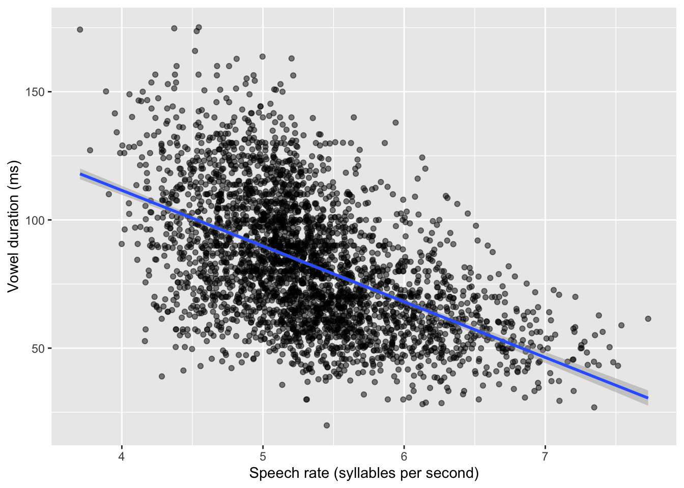

Figure 24.1: Scatter plot of speech rate (as number of syllables per second) and vowel duration (in milliseconds) in 19 Italian speakers.

You might be wondering what is the warning about missing values. This is because some observations of vowel duration (v1_duration) in the data are missing (i.e. they are NA, “Not Available”). We can drop them from the tibble using drop_na(). This function takes column names as arguments: each row that has NA in any of the columns listed in the function will be dropped, so be careful when using drop_na() without listing columns because any NA value in any column with make the row be removed.

ita_egg_clean <- ita_egg |> 
  drop_na(v1_duration)

We will use ita_egg_clean for the rest of the tutorial. Let’s reproduce the plot, but let’s add a regression line. This is the straight line we have been talking about, the line that is reconstructed by regression models. It is sometimes useful to add the regression line to the scatter plots to show the linear relationship of the two variables in the plot. We can quickly add regression lines to scatter plots with the smooth geometry: geom_smooth(method = "lm"). The method argument lets us pick the type of method to create the “smooth”: here, we want a regression line so we choose lm for linear model (remember, linear model is another term for regression model). Under the hood, geom_smooth() fits a regression model to estimate the regression line and plots it. We will fit our own regression model below, so for now the regression line is just for show. Figure 24.2 shows the scatter plot with the regression line. You can ignore the message about the formula.

ita_egg_clean |> 
  ggplot(aes(speech_rate, v1_duration)) +
  geom_point(alpha = 0.5) +
  geom_smooth(method = "lm") +
  labs(
    x = "Speech rate (syllables per second)",
    y = "Vowel duration (ms)"
  )

`geom_smooth()` using formula = 'y ~ x'

Figure 24.2: Relationship between speech rate (as number of syllables per second) and vowel duration (in milliseconds) in 19 Italian speakers.

By glancing at the individual points, we can see a negative relationship between speech rate and vowel duration: vowels get shorter with greater speech rate. This is reflected by the regression line too, which has a negative slope. A negative slope means that when the values on the x-axis increase, the values on the y-axis decrease. When the opposite is true, i.e. when with increasing x-axis values you observe increasing y-axis values, we say the regression line has positive slope. Positive and negative slope correspond to what some call a direct and inverse relationship. In terms of the equation of the line \(y = \beta_0 + \beta_1 x\), a positive slope means \(\beta_1\) is a positive number and, conversely, a negative slope means \(\beta_1\) is a negative number. When \(\beta_0\) is zero, then the regression line is flat and we say that the two variables are independent: changing one, does not systematically change the other. You explored these features of the regression slope in Chapter 23, when playing around with the Regression Models Illustrated app and when answering the quiz.

Direct/positive and inverse/negative relationship

When the slope \(\beta_1\) is positive, the regression line has positive slope and \(x\) and \(y\) have a direct relationship.

When the slope \(\beta_0\) is negative, the regression line has negative slope and \(x\) and \(y\) have an inverse relationship.

When the slope \(\beta_0\) is 0 zero, the regression line is flat and \(x\) and \(y\) are independent.

Figure 24.2 looks very nice, but the plot doesn’t tell us much about the estimates for \(\beta_0\) and \(\beta_1\). For that, we need to actually fit the regression model.

24.1.1 The model

Let’s move on onto fitting a Gaussian regression model to vowel duration as the outcome variable and speech rate as the predictor. We are assuming that vowel duration follows a Gaussian distribution (although as mentioned at the beginning of this chapter, this is not the case, but it will do for now). Here is the model we will fit, in mathematical notation.

\[ \begin{align} vdur & \sim Gaussian(\mu, \sigma)\\ \mu & = \beta_0 + \beta_1 \cdot sr\\ \end{align} \]

You can read that as:

• Vowel duration (\(vdur\)) is distributed (\(\sim\)) according to a Gaussian distribution (\(Gaussian(\mu, \sigma)\)).

• The mean \(\mu\) is equal to the sum of \(\beta_0\) (the intercept) and the product of \(\beta_1\) and speech rate (\(\beta_1 \cdot sr\)). The formula of \(\mu\) is regression equation of the model.

The regression model estimates the parameters in the mathematical formulae: the parameters to be estimated in regression models are usually represented with Greek letters (hence why we adopted this notation for the linear equation). The regression model in the formulae above has to estimate the following three parameters:

• The regression coefficients \(\beta_0\) and \(\beta_1\).

• The standard deviation of the Gaussian distribution, \(\sigma\).

\(\beta_0\) and \(\beta_1\) are called the regression coefficients because they are coefficients of the regression equation. In maths, a coefficient is simply a constant value that multiplies a “basis” in the equation, like the variable \(sr\). In the regression equation of the model, \(\beta_1\) is a multiplier of the variable \(sr\), but what about \(\beta_0\)? Well, it is implied that \(\beta_0\) is a multiplier of the constant basis 1, because \(\beta_0 \cdot 1 = \beta_0\). Knowing this should now reveal the reason behind the strange formula that R uses in Gaussian models like the ones we fitted in Chapter 22: the 1 in the formula stands for the constant basis of the intercept, meaning that the model estimates the coefficient of the intercept, \(\beta_0\). Gaussian models without predictors are in fact also called intercept-only regression models, because only an intercept is estimated. There is no slope in the model because there is not variable \(x\) to multiply the slope with.

Going back to our regression model of vowel duration and speech rate, we can rewrite the model formula to make the constant basis 1 explicit, thus:

\[ \begin{align} vdur & \sim Gaussian(\mu, \sigma)\\ \mu & = \beta_0 \cdot 1 + \beta_1 \cdot sr\\ \end{align} \]

To instruct R to model vowel duration as a function of the numeric predictor speech rate you simply add it to the 1 we have used in the right-hand side of the tilde in Chapter 22 (i.e. v1_duration ~ 1): so v1_duration ~ 1 + speech_rate. The R formula is based on the bases you multiply the coefficients with in the mathematical formula: \(1\) and \(sr\). In R parlance, the 1 and sr in the R formula are called predictor terms, or terms for short. While the predictor \(sr\) can take different values, the \(1\) is constant so it is also called the constant term, or the intercept term (because it is the basis of the intercept \(\beta_0\)). In the R formula, you don’t explicitly include the coefficients \(\beta_0\) and \(\beta_1\), just the bases. Put all this together and you get the 1 + speech_rate part of the formula. There is more: in R, since the \(1\) is a constant, you can omit it! So v1_duration ~ 1 + speech_rate can also be written as v1_duration ~ speech_rate. They are equivalent.

That was probably a lot! But now that we have clarified how the R formula is set up, we can proceed and fit the model. Here is the full code to fit a Gaussian regression model of vowel duration with brms.

library(brms)

vow_bm <- brm(
  # `1 +` can be omitted.
  v1_duration ~ 1 + speech_rate,
  # v1_duration ~ speech rate,
  family = gaussian,
  data = ita_egg_clean
)

R Note: The rethinking package

McElreath’s textbook Statistical Rethinking (McElreath 2020) comes with an R package, rethinking, that lets you fit data using R formulae that resemble the mathematical formulae more closely. For example, in rethinking the model formula of our model of vowel duration would look like the code below. The package requires you to include all the formulae in a list. Note that the rethinking package does not set default priors, so we have included them below.

alist(
  v1_duration ~ dnorm(mu, sigma),
  mu <- b0 + b2 * speech_rate,
  # Priors
  a ~ dt(80, 25), 
  b ~ dt(0, 1),
  sigma ~ dt(0, 25)
)

If you look closely at the the first two lines in the list, you should recognise the mathematical formulae of the model we have seen above.

24.2 Interpret the model summary

As we has seen in Chapter 22, to obtain a summary of the model, we use the summary() function.

summary(vow_bm)

 Family: gaussian 
  Links: mu = identity; sigma = identity 
Formula: v1_duration ~ speech_rate 
   Data: ita_egg_clean (Number of observations: 3253) 
  Draws: 4 chains, each with iter = 2000; warmup = 1000; thin = 1;
         total post-warmup draws = 4000

Regression Coefficients:
            Estimate Est.Error l-95% CI u-95% CI Rhat Bulk_ESS Tail_ESS
Intercept     198.47      3.33   191.76   204.97 1.00     3681     2274
speech_rate   -21.73      0.62   -22.93   -20.49 1.00     3623     2421

Further Distributional Parameters:
      Estimate Est.Error l-95% CI u-95% CI Rhat Bulk_ESS Tail_ESS
sigma    21.66      0.27    21.14    22.19 1.00     3855     2615

Draws were sampled using sampling(NUTS). For each parameter, Bulk_ESS
and Tail_ESS are effective sample size measures, and Rhat is the potential
scale reduction factor on split chains (at convergence, Rhat = 1).

Let’s focus on the Regression Coefficients table of the summary. It should now be clear why in the summary of the model in Chapter 22, the summaries for the mean \(\mu\) (i.e. \(\beta_0\)) were in the regression coefficients table. The table of the regression model we just fit has two coefficients. To understand what they are, just remember the equation of the line and the model formula above, repeated here.

\[ \begin{align} vdur & \sim Gaussian(\mu, \sigma)\\ \mu & = \beta_0 \cdot 1 + \beta_1 \cdot sr\\ \end{align} \]

• Intercept is \(\beta_0\): this is the mean vowel duration, when speech rate is 0.

• speech_rate is \(\beta_1\): this is the change in vowel duration for each unit increase of speech rate.

This should make sense, if you understand the equation of a line: \(y = \beta_0 + \beta_1 x\). Remember, the intercept \(\beta_0\) is the \(y\) value when \(x\) is 0. In our regression model, \(y\) is vowel duration \(vdur\) and \(x\) is speech rate \(sr\). So the Intercept is the mean vowel duration when speech rate is 0. Recall that the Estimate and Est.Error column are simply the mean and standard deviation of the posterior probability distributions of the estimate of Intercept and speech_rate respectively. In this model we just have two coefficients instead of one. Looking at the 95% Credible Intervals (CrIs), we can say that based on the model and data:

• The mean vowel duration, when speech rate is 0 syl/s, is between 192 and 205 ms, at 95% confidence.

• We can be 95% confident that, for each unit increase of speech rate (i.e. for each increase of one syllable per second), the duration of the vowel decreases by 20.5-23 ms.

To answer our research question (what is the relationship between vowel duration and speech rate?) we can say that with increasing speech rate, vowel duration decreases. We can be more precise than that and say that for each increase of one syllable per second, the vowel becomes 20.5 to 23 ms shorter, at 95% confidence (that is our 95% CrI). Since this is a regression model, it doesn’t matter if we are comparing \(vdur\) when \(sr = 0\) vs when \(sr = 1\), or when \(sr = 6.5\) vs when \(sr = 7.5\). The slope coefficient \(\beta_1\) tells us what to add to \(vdur\) when you increase \(sr\) by one. For example, assume you want to obtain from the model an estimate of mean \(vdur\) when speech rate is 5. You would just plug in \(sr = 5\) in the formula:

\[ \begin{align} \mu & = \beta_0 + \beta_1 \cdot 5\\ \end{align} \]

So that is the intercept \(\beta_0\) plus \(\beta_1\) times the speech rate, i.e. 5. The only complication is that here \(\beta_0\) and \(\beta_1\) are full probability distributions, rather than single values like you would have in the simple case of the equation of a line. Since the coefficients are posterior probability distributions, any operation like addition and multiplication will lead to a posterior probability distribution, i.e. the posterior probability distribution of \(\mu\). You will learn how do to these operations in the next chapter, Chapter 25.

For now, let’s focus on the posterior distributions of the coefficients. To see what the posterior probability densities of \(\beta_0\), \(\beta_1\) and \(\sigma\) look like, you can quickly plot them with the plot() function, as we did in Chapter 22. There is also another way: we can use the mcmc_dens() function from the bayesplot package (why it’s mcmc_dens() will become clear in Chapter 25). By default the function plots the posterior densities of all parameters in the model, plus other internal parameters that we usually don’t care about. We can conveniently specify which parameters to plot with the pars argument, which takes a character vector. The names of the parameters for the regression coefficients are slightly different than what you see in the summary: b_Intercept and b_speech_rate. These are just the names you see in the summary, with a prefixed b_. The b_ stands for beta coefficient, which makes sense, since these are the \(\beta_0\) and \(\beta_1\) coefficients. Figure 24.3 shows the output of the mcmc_dens() function.

library(bayesplot)

mcmc_dens(vow_bm, pars = c("b_Intercept", "b_speech_rate", "sigma"))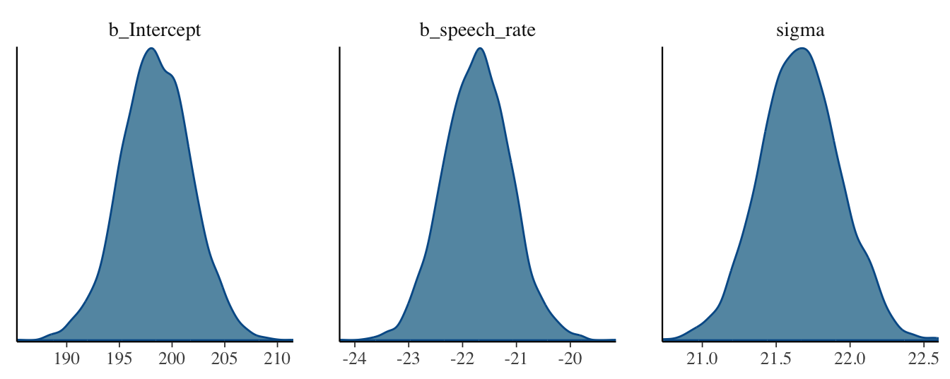

Figure 24.3: Posterior density plots of a regression model fitted to vowel duration.

These are the results of the regression model: the full posterior probability distributions of the three parameters \(\beta_0\), \(\beta_1\), \(\sigma\). The posteriors can be described, as with any other probability distribution, by the values of their parameters. It is common to use the mean and standard deviation, the parameters of the Gaussian distribution. This is independent from the fact that we fitted a Gaussian distribution: posterior distributions tend to be bell-shaped, i.e. Gaussian. This is why the Regression Coefficients table of the summary reports mean and SD, i.e. Estimate and Est.Err, as mentioned earlier.

You should always also plot the model predictions, i.e. the predicted values of vowel duration based on the model predictors (here just speech_rate). You will learn more advanced methods later on, but for now you can use conditional_effects() from the brms package.

conditional_effects(vow_bm, effects = "speech_rate")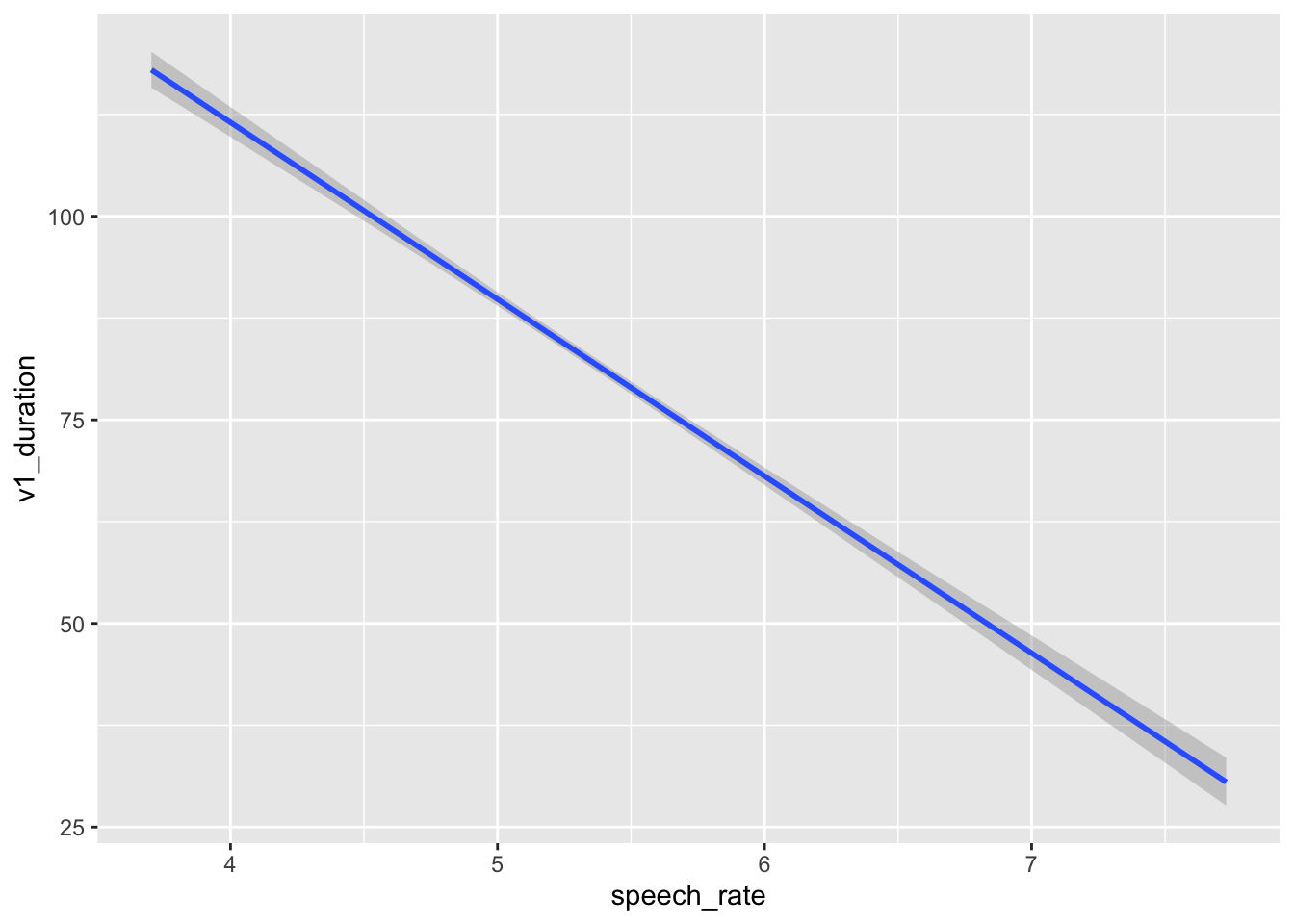

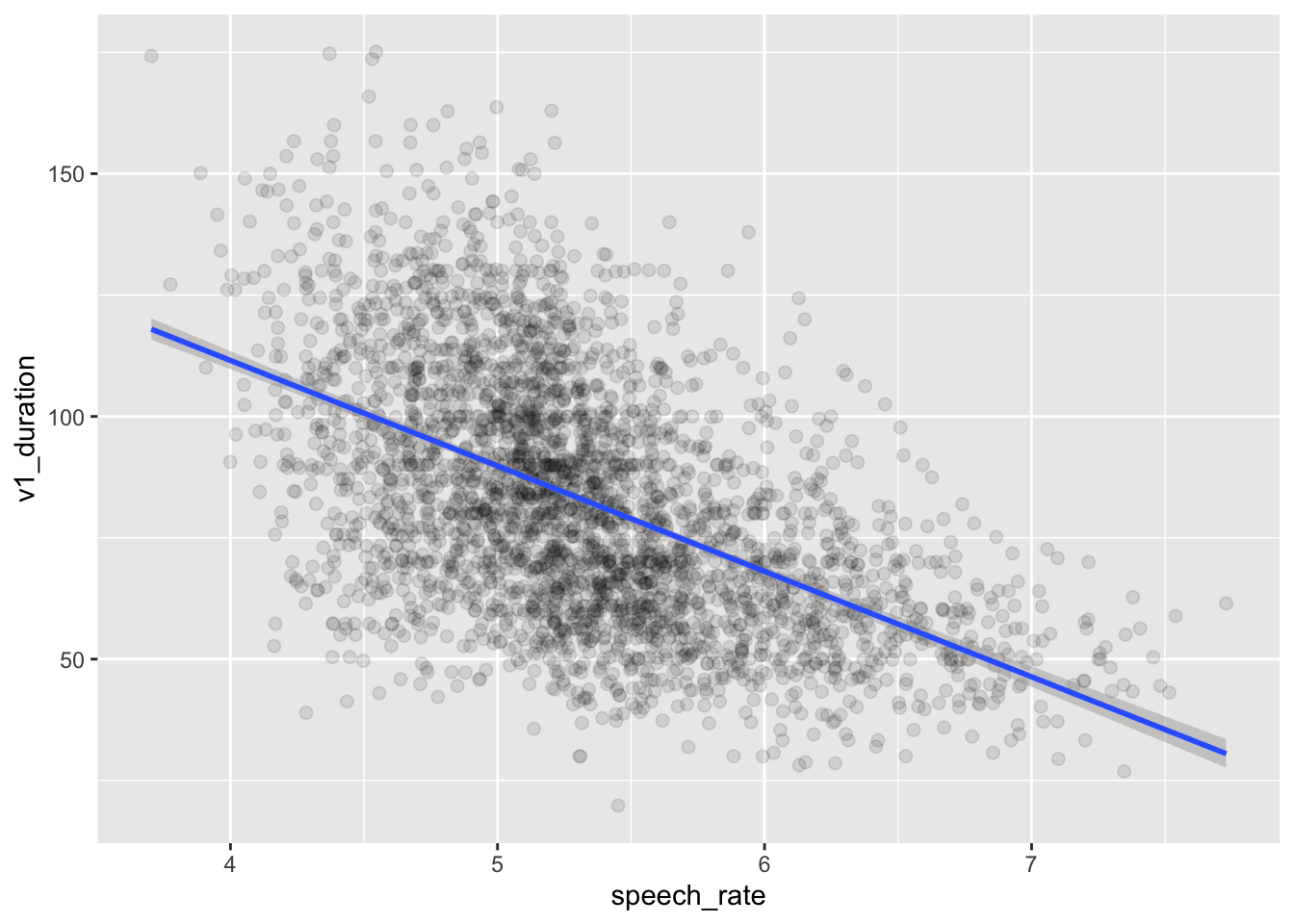
Figure 24.4: Posterior predictions of vowel duration based on speech rate from a regression model.

If you wish to include the raw data in the plot, you can wrap conditional_effects() in plot() and specify points = TRUE. Any argument that needs to be passed to geom_point() (these are all ggplot2 plots!) can be specified in a list as the argument point_args. Here we are making the points transparent.

plot(
  conditional_effects(vow_bm, effects = "speech_rate"),
  points = TRUE,
  point_args = list(alpha = 0.1)
)

Figure 24.5: Posterior predictions of vowel duration based on speech rate from a regression model (repr.).

This plot looks basically the same as Figure 24.2. Indeed, in Figure 24.2 we used geom_smooth() to add a regression line from a regression model. A warning told us that this formula was used: y ~ x. In the context of that plot, that means the smooth function fitted a regression model with speech rate as x and vowel duration as y. This is because the aesthetics are exactly aes(x = speech_rate, y = v1_duration) (we didn’t write the x = and y = because they are implied). So geom_smooth() has fitted exactly the same model we have fitted with brms. It might look trivial to fit a full model when you can just look at the regression line of geom_smooth(). This is not the case for two reasons: first, you just see a regression line, but you don’t know what the posterior distributions of the parameters are; second, with more complex scenarios, geom_smooth() falls short and can only produce regression lines based on very simple formulae like y ~ x.¹

24.3 Reporting

You have seen an example of reporting in Chapter 22. We can use that as a template for reporting a regression model, by reworking a few parts and adding information related to the numeric predictor in the regression. You could report the vowel duration regression model like so:

We fitted a Bayesian regression model using the brms package (Bürkner 2017) in R (R Core Team 2025). We used a Gaussian distribution for the outcome variable, vowel duration (in milliseconds). We included speech rate (measured as syllables per second) as the regression predictor.

Based on the model results, there is a 95% probability that the mean vowel duration, when speech rate is 0, is between 192 and 205 ms (mean = 198, SD = 3). For each unit increase of speech rate (i.e. for each one syllable per second added), vowel duration decreases by 20 to 23 ms (mean = -22, SD = 1). The residual standard deviation is between 21 and 22 ms (mean = 22, SD = 0).

Note the wording of the speech rate coefficient: “vowel duration decreases by 20 to 23 ms”. The speech rate coefficient 95% CrI is fully negative (i.e. both lower and upper limit are negative) so we can say that vowel duration decreases. Furthermore, since we say “decreases” then we should report the CrI limits as positive numbers. Think about it: we say “decrease X by 2” to mean “X - 2”, rather than “decrease X by -2”. Finally, given we flipped the signs of the CrI limits, it is clearer to write “20 to 23 ms”, rather than the other way round as you would if you reported the interval as is: 95% CrI [-23, -20].

Another point to note is that in the reporting style I am using in this book, we place more emphasis on the posterior CrI than on the posterior mean and SD. So the CrI is in the main text, while mean and SD are between parentheses. Other researchers might in fact do it the other way round. Whatever you decide to do, be consistent. Finally, it is unusual to report the coefficients of \(\sigma\): I have done it here for completeness, since it doesn’t hurt to do so.

24.4 What’s next

In this chapter you have learned the very basics of Bayesian regression models. As mentioned above, regression models with brms are very flexible and you can easily fit very complex models with a variety of distribution families (for a list of available families, see ?brmsfamily; you can even define your own distributions!). The perk of using brms is that you can just learn the basics of one package and one approach and use it to fit a large variety of regression models. This is different from the standard frequentist approach, where different models require different packages or functions, with their different syntax and quirks. In the following weeks, you will build your understanding of Bayesian regression models, which will enable you to approach even the most complex models! However, due to time limits you won’t learn everything there is to learn in this course. Developing conceptual and practical skills in quantitative methods is a long-term process and unfortunately one semester will not be enough. So be prepared to continue your learning journey for years to come!

24.5 Summary

• Gaussian regression models have the following mathematical form:

\[ \begin{align} y & \sim Gaussian(\mu, \sigma)\\ \mu & = \beta_0 + \beta_1 x\\ \end{align} \]

• A regression model estimates an intercept \(\beta_0\) and a slope \(\beta_1\) from the data (\(x\) and \(y\)).

• Regression models in brms are fit with the R formula y ~ 1 + x. We can omit the constant/intercept term: y ~ x.

• The intercept \(\beta_0\) is the mean \(y\) when \(x\) is 0 zero.

• The slope \(\beta_1\) is the change in \(y\) for every unit increase of \(x\).

Bürkner, Paul-Christian. 2017. “Brms: An r Package for Bayesian Multilevel Models Using Stan.” Journal of Statistical Software 80 (1): 128. https://doi.org/10.18637/jss.v080.i01.

Coretta, Stefano. 2019. “Vowel Duration, Voicing Duration, and Vowel Height: Acoustic and Articulatory Data from Italian [Research Compendium].” https://doi.org/10.17605/OSF.IO/XDGFZ.

McElreath, Richard. 2020. Statistical Rethinking: A Bayesian Course with Examples in R and Stan. Second edition. Chapman & Hall/CRC Texts in Statistical Science Series. Boca Raton: CRC Press.

R Core Team. 2025. R: A Language and Environment for Statistical Computing [Version 4.5.0].

Winter, Bodo. 2020. Statistics for Linguists: An Introduction Using r. Routledge.

---

1. Technically, geom_smooth() uses lm() under the hood. This is a base R function that fits regression models using maximum likelihood estimation (MLE). This way of estimating regression coefficients is common in frequentist approaches to regression modelling and we will not treat it here. If you are interested about lm() and MLE, you can learn about these in Winter (2020).