mald <- readRDS("data/tucker2019/mald_1_1.rds")
mald27 Regression with categorical predictors
![]()
![]()
In Chapter 24 you learned how to fit regression models of the following form in R using the brms package.
\[ \begin{aligned} y & \sim Gaussian(\mu, \sigma)\\ \mu & = \beta_0 + \beta_1 \cdot x\\ \end{aligned} \]
In these models, \(x\) was a numeric predictor, like speech rate in the chapter’s example. Numeric predictors are not the only type of predictors that a regression model can handle. Regression predictors can also be categorical variables: gender, age group, place of articulation, mono- vs bi-lingual, etc. However, regression model cannot handle categorical predictors directly: think about it, what would it mean to multiply \(\beta_1\) by “female” or by “old”? Categorical predictors have to be re-coded as numbers.
In this chapter we will revisit the MALD reaction times (RTs) data from Chapter 22, this time with the following research question:
Is the RTs in a auditory lexical decision task affected by the type of the target word (real or not)?
This chapter will teach you the default way of including categorical predictors in regression models: numerical coding with treatment contrasts. This is the most common way to code categorical predictors.
27.1 Revisiting reaction times
Let’s read the MALD data (Tucker et al. 2019). The data contains reaction times from an auditory lexical decision task with English listener: the participants would hear a word (real or not) and would have to press a button to say if the word was a real English word or not.
The relevant columns are RT with the RTs in milliseconds and IsWord, the type of target word: it tells if the target word the listeners heard is a real English word (TRUE) or not (a nonce word, FALSE). Figure 27.1 shows the density plot of RTs, grouped by whether the target word is real or not. We can notice that the distribution of RTs with nonce (non-real) words is somewhat shifted towards higher RTs, indicating that more time is needed to process nonce words than real words.
Code
mald |>
  ggplot(aes(RT, fill = IsWord)) +
  geom_density(alpha = 0.8) +
  geom_rug(alpha = 0.1) +
  scale_fill_brewer(palette = "Dark2")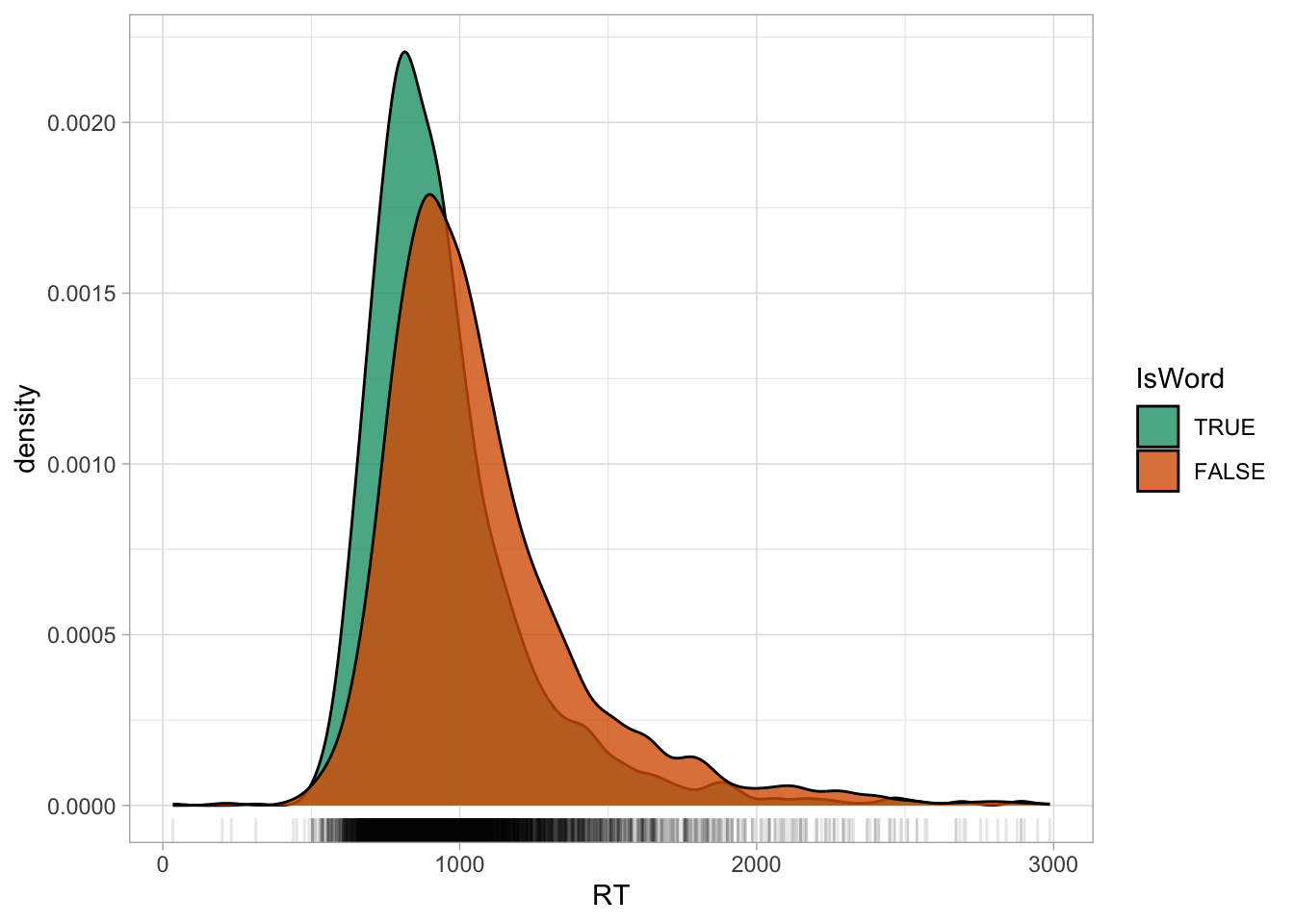
You might also notice that the “tails” of the distributions (the left and right sides) are not symmetric: the right tail is heavier that the left tail. This is a very common characteristics of RT values and of any variable that can only be positive (like vowel duration or the duration of any other phonetic unit). These variables are “bounded” to only positive numbers. You will learn later on that the values in these variables are generated by a log-normal distribution ( Chapter 31), rather than by a Gaussian distribution (which is “unbounded”). For the time being though, we will model the data as if they were generated by a Gaussian distribution, so that we can focus on the categorical predictor part.
Another way to present a numeric variable like RTs depending on categorical variables is to use a jitter plot, like Figure 27.2. A jitter plot places dots corresponding to the values in the data on “strips”. The strips are created by randomly jittering dots horizontally, so that they don’t all fall on a straight line. The width of the strips, aka the jitter, can be adjusted with the width argument. It’s subtle, but you can see how in the range 1 to 2 seconds there are a bit more dots in nonce words (right, orange) than in real words (left, green). In other words, the density of dots in that range is greater in nonce words than real words. If you compare again the densities in Figure 27.1 above, you will notice that the orange density in the 1-2 seconds range is higher in nonce words. These are just two ways of visualising the same thing.
mald |>
  ggplot(aes(IsWord, RT, colour = IsWord)) +
  # width controls the width of the strip with jittered points
  geom_jitter(alpha = 0.15, width = 0.1) +
  scale_colour_brewer(palette = "Dark2")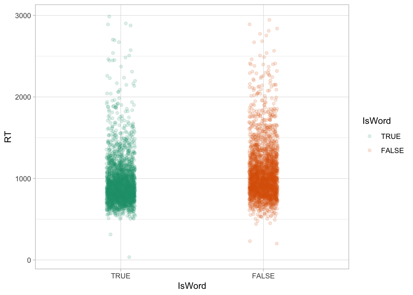
We can even overlay density plots on jitter plots using “violins”, like in Figure 27.3. The violins are simply mirrored density plots, placed vertically on top of the jittered strips. The width of the violins can be adjusted with the width argument, like with the jitter.
mald |>
  ggplot(aes(IsWord, RT, fill = IsWord)) +
  geom_jitter(alpha = 0.15, width = 0.1) +
  geom_violin(width = 0.2) +
  scale_fill_brewer(palette = "Dark2")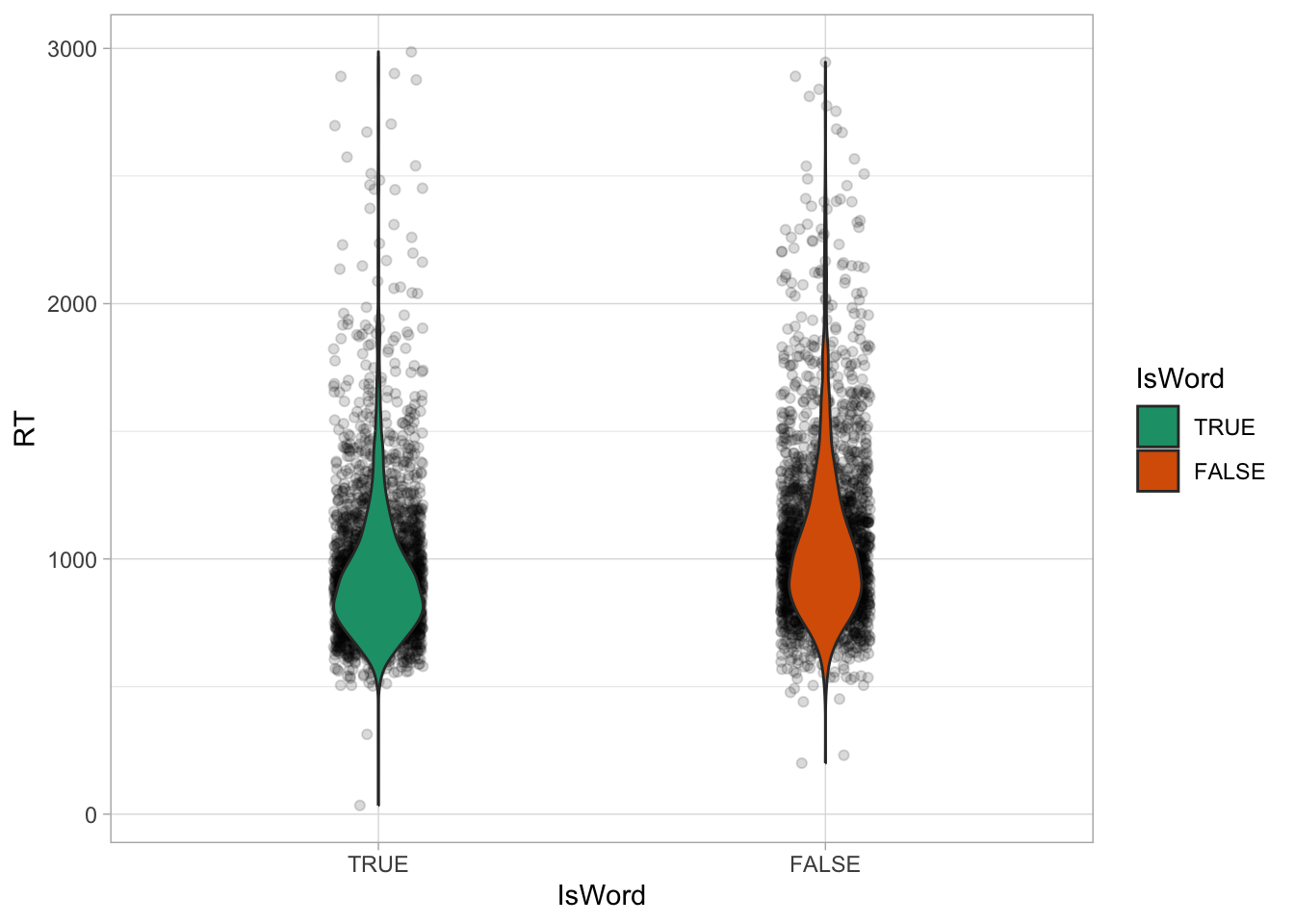
It is good practice to show the raw data and the density using violin and jitter plots, because patterns in the data are visible when plotting the raw data (while they aren’t when using for example bar charts, more on this in Section 30.3), so this should be your go-to choice for plotting numeric data by categorical groups, like RTs and type of word here. Now we can obtain a few summary measures. The following code groups the data by IsWord and then calculates the mean, median and standard deviation of RTs. After summarise(), we are using a trick to round all columns that are numeric, namely the columns with the mean, median and SD. The trick is to use the across() function in combination of where(). across(where(is.numeric), round) means “across columns where the type is numeric, round the value”.
mald_summ <- mald |>
  group_by(IsWord) |>
  summarise(
    mean(RT), median(RT), sd(RT)
  ) |>
  mutate(
    # round all numeric columns
    across(where(is.numeric), round)
  )

mald_summ
The mean and median RTs for nonce words (IsWord = FALSE) are about 100 ms higher than the mean and median of real words. We could stop here and call it a day, but we would make the mistake of not considering uncertainty and variability: this is just one (admittedly large) sample of all the RT values that could be produced by the entire English-speaking population. So we should apply inference from the sample to the population to obtain an estimate of the difference in RTs that accounts for that uncertainty and variability. We can use regression models to do that. The next sections will teach you how to model the RTs with regression models in brms.
27.2 Treatment contrasts
We can model RTs with a Gaussian distribution (although as mentioned above, this family of distribution is generally not appropriate for variables liker RTs) with a mean \(\mu\) and a standard deviation \(\sigma\): \(RT \sim Gaussian(\mu, \sigma)\). This time though we want to model a different mean \(\mu\) depending on the word type in IsWord. How do we make the model estimate a different mean depending on IsWord? There are several ways of setting this up. The default method is to use so-called treatment contrasts which involves numerical coding of categorical predictors (the coding takes the same naming as the contrasts, so the coding for treatment contrasts is treatment coding). Let’s work by example with IsWord. This is a categorical predictor with two levels: TRUE and FALSE. With treatment contrasts, one level is chosen as the reference level and the other is compared to the reference level. The reference level is automatically set as the first level in the predictor in alphabetical order. This would mean that FALSE would be the reference level, because “F” comes before “T”.
However, in the mald data, the column IsWord is a factor column and the levels have been ordered so that TRUE is the first level and FALSE the second. You can see this in the Environment panel, if you click on the arrow next to mald and look next to IsWord: it will say Factor w/ 2 levels "TRUE","FALSE". You can also check the order of the levels of a factor with the levels() function.
levels(mald$IsWord)[1] "TRUE" "FALSE"You can set the order of the levels with the factor() function. If you don’t specify the order of the levels, the alphabetical order will be used. For example:
fac <- tibble(
  fac = c("a", "a", "b", "b", "a"),
  fac_1 = factor(fac),
  fac_2 = factor(fac, levels = c("b", "a"))
)

levels(fac$fac_1)
[1] "a" "b"levels(fac$fac_2)[1] "b" "a"We will use IsWord with the order TRUE and FALSE. This means that TRUE will be the reference level and the RTs when IsWord is FALSE will be compared to the RTs of when IsWord is TRUE. In other words, now the mean \(\mu\) varies depending on the level of IsWord. We need to numerically code IsWord (i.e. use numbers to refer to the levels of the categorical predictor) to be able to allow the mean to vary by the word type in the model formula. With treatment contrasts, treatment coding is used to numerically code categorical predictors. Treatment coding uses indicator variables which take the values 0 or 1. Let’s make an indicator variable \(w\) that is 0 when IsWord is TRUE, or 1 when IsWord is FALSE. We only need one indicator variable because there are only two levels and they can be coded with a 0 and a 1 respectively. This way of setting up indicator variables (using 0/1) is called dummy coding. See Table 27.2 for the correspondence between the predictor IsWord and the value of the indicator variable \(w\).
IsWord.
IsWord |
\(w\) |
|---|---|
| IsWord = TRUE | 0 |
| IsWord = FALSE | 1 |
We can now update the equation of \(\mu\):
\[ \begin{aligned} RT_i & \sim Gaussian(\mu_i, \sigma)\\ \mu_i & = \beta_0 + \beta_1 \cdot w_i\\ \end{aligned} \]
The subscript \(i\) is an index of each observation in the data. There are 5000 observations in mald so \(i = [1..5000]\) (\(i\) goes from 1 to 5000). \(RT_i\) then is indexing the specific observations in the data, \(RT_1\), \(RT_2\), \(RT_3\), …, \(RT_{5000}\). Each observation is from a real or nonce word: this is coded by \(w_i\). The subscript \(i\) in \(w_i\) is indexing the IsWord value of the \(i\)th observation. In the data, \(RT_1 = 617\) and \(w_1 = 0\) (i.e. TRUE). The mean \(\mu_i\) also has a subscript \(i\). The \(i\) is there to say that now \(\mu\) depends on the specific observation \(i\), so that we can model a different mean depending on \(w_i\). In fact, in the model in Chapter 24, \(i\) was implied to keep things simple, but technically it should be added, because the mean does depend on the value of \(w\):
\[ \begin{aligned} RT_i & \sim Gaussian(\mu_i, \sigma)\\ \mu_i & = \beta_0 + \beta_1 \cdot w_i\\ \end{aligned} \]
These are just technicalities of the notation, so you shouldn’t get too caught up on it, the substance of the model is the same.
Going back to our model of RTs as a function of word type (“as a function of” is another way of saying that you are modelling an outcome variable depending on a predictor), \(\beta_0\) and \(\beta_1\) are the regression coefficients, exactly like in the regression model with vowel duration and speech rate. You can think of \(\beta_0\) as the model’s intercept and of \(\beta_1\) as the model’s slope. Can you figure out why? Recall that a regression model with a numeric predictor is basically the formula of a line. In Chapter 24, we modelled vowel duration as a function of speech rate. The intercept of the regression line estimated by the model indicates where the line crosses the y-axis when the x value is 0: in that model, that was the vowel duration when speech rate is 0. In the model above, with RTs as a function of word type, the numeric predictor is the indicator variable \(w\), which stands for the categorical predictor IsWord. The formula of a line really works just with numbers so for the formula to make sense, we had to make the categorical predictor IsWord into a number and treatment contrasts is such one way of doing so.
Now, \(\beta_0\) is the model’s intercept because that is the mean RT when \(w\) is 0 (like with vowel duration when speech rate is 0; can you see the parallel?). And \(\beta_1\) is the model’s slope because \(\beta_1\) is the change in RT for a unit increase of \(w\), which is when \(w\) goes from 0 to 1. This in turn corresponds to the change in level in the categorical predictor. Do you see the connection? It’s a bit contorted, but once you get this, it should explain several aspects of regression models with categorical predictors and treatment contrasts. So \(\mu_i\) is the sum of \(\beta_0\) and \(\beta_1 \cdot w_i\). \(w_i\) is 0 (when the word is real) or 1 (the the word is a nonce word). That is why we write \(RT_i\): the subscript \(i\) allows us to pick the correct value of \(w_i\) for each specific observation. The result of plugging in the value of \(w_i\) is laid out in the following formulae.
\[ \begin{aligned} \mu_i & = \beta_0 + \beta_1 \cdot w_i\\ \mu_{\text{T}} & = \beta_0 + \beta_1 \cdot 0 = \beta_0\\ \mu_{\text{F}} & = \beta_0 + \beta_1 \cdot 1 = \beta_0 + \beta_1 \end{aligned} \]
When
IsWordisTRUE, the mean RT is equal to \(\beta_0\).When
IsWordisFALSE, the mean RT is equal to \(\beta_0 + \beta_1\).
If \(\beta_0\) is the mean RT when IsWord is TRUE, what is \(\beta_1\) by itself? Simple.
\[ \begin{aligned} \beta_1 & = \mu_\text{F} - \mu_\text{T}\\ & = (\beta_0 + \beta_1) - \beta_0 \end{aligned} \]
\(\beta_1\) is the difference between the mean RT when IsWord is TRUE and the mean RT when IsWord is FALSE. As mentioned above, with treatment contrasts you are comparing the second level to the first. So one regression coefficient will be the mean of the reference level, and the other coefficient will be the difference between the mean of the two levels. I know this is not particularly beginner-friendly, but this is the default in R when using categorical predictors and it is the most common way to code categorical predictors, so you will frequently find tables in academic articles with regression coefficients that have to be interpreted that way.
27.3 Model RTs by word type
That was a lot of theory, so let’s move onto the application of that theory. Fitting a regression model with a categorical predictor like IsWord is as simple as including the predictor in the model formula, to the right of the tilde ~. From now on we will stop including 1 + since an intercept term is always included by default.
rt_bm_1 <- brm(
  # equivalent: RT ~ 1 + IsWord
  RT ~ IsWord,
  family = gaussian,
  data = mald,
  seed = 6725,
  file = "cache/ch-regression-cat-rt_bm_1"
)
Treatment contrasts are applied by default: you do not need to create an indicator variable yourself or tell brms to use that coding (which is both a blessing and a curse). The following code chunk returns the summary of the model rt_bm_1.
summary(rt_bm_1) Family: gaussian
Links: mu = identity; sigma = identity
Formula: RT ~ IsWord
Data: mald (Number of observations: 5000)
Draws: 4 chains, each with iter = 2000; warmup = 1000; thin = 1;
total post-warmup draws = 4000
Regression Coefficients:
Estimate Est.Error l-95% CI u-95% CI Rhat Bulk_ESS Tail_ESS
Intercept 953.14 6.12 941.17 965.17 1.00 4590 2897
IsWordFALSE 116.34 8.80 98.74 134.14 1.00 4815 3235
Further Distributional Parameters:
Estimate Est.Error l-95% CI u-95% CI Rhat Bulk_ESS Tail_ESS
sigma 312.47 3.11 306.44 318.60 1.00 4720 3456
Draws were sampled using sampling(NUTS). For each parameter, Bulk_ESS
and Tail_ESS are effective sample size measures, and Rhat is the potential
scale reduction factor on split chains (at convergence, Rhat = 1).The first few lines should be familiar: they report information about the model, like the distribution family, the formula, the MCMC draws and so on. Then we have the Regression Coefficients table, just like in the model of Chapter 24. The estimates of the coefficients and the 95% Credible Intervals (CrIs) are reported in Table 27.3 (the table was generated with knitr::kable() from the R Note above! Expand the code to see it).
Code
fixef(rt_bm_1) |> knitr::kable()| Estimate | Est.Error | Q2.5 | Q97.5 | |
|---|---|---|---|---|
| Intercept | 953.1412 | 6.120423 | 941.16925 | 965.1697 |
| IsWordFALSE | 116.3413 | 8.800872 | 98.73942 | 134.1424 |
Just to remind you: the Estimate column is the mean of the posterior distribution of the regression coefficients, and Est.Error is the standard deviation of the posterior distribution of the regression coefficients. Q2.5 and Q97.5 are the lower and upper limit of the 95% CrI of the posterior distribution of the regression coefficients. Let’s plot the posterior distributions of the two coefficients.
Code
mcmc_dens(rt_bm_1, pars = vars(starts_with("b_")))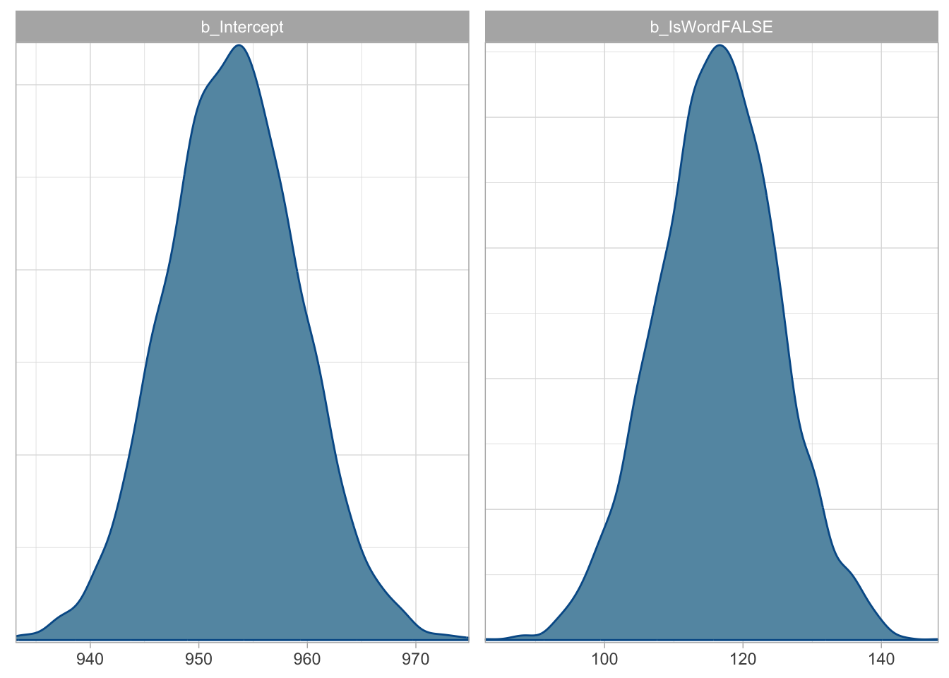
rt_bm_1.
b_Intercept(Interceptin the model summary) is the mean RT whenIsWordisTRUE. This is \(\beta_0\) in the model’s mathematical formula.b_IsWordFALSE(IsWordFALSEin the model summary) is the difference in mean RT between nonce and real words. This is \(\beta_1\) in the model’s mathematical formula.
Moving onto the 95% CrIs:
The 95% CrI of
Intercept\(\beta_0\) is [941, 965] ms: this means that there is a 95% probability that the mean RT whenIsWordisTRUEis between 941 and 965 ms.The 95% CrI of
IsWordFALSE\(\beta_0\) is [99, 134] ms: this means that there is a 95% probability that the difference in mean RT between nonce and real words is between 99 and 134 ms.
So here we have our answer: at 95% confidence (another way of saying at 95% probability), based on the model and data, RTs for nonce words are 99 to 134 ms longer than RTs for real words. What about the expected RTs for nonce words?
27.4 Expected predictions
The coefficients are just telling us the difference in RT between nonce and real words, but not the expected mean RT for nonce words. As in Chapter 25, we can simply plug in the draws from the model according to the model formulae to obtain any estimand of interest, like the expected value of RTs when the word is not a real word. Remember, for nonce words (\(w_i = 1\)):
\[ \begin{aligned} \mu_{\text{F}} & = \beta_0 + \beta_1 \cdot 1 = \beta_0 + \beta_1 \end{aligned} \]
To get the expected RTs for nonce words we need to sum b_Intercept and b_IsWordFALSE. While we are at it, we also create a column for real words (that is just b_Intercept so we are basically just copying it that column; remember, \(\mu_T = \beta_1\)).
rt_bm_1_draws <- as_draws_df(rt_bm_1) |>
  mutate(
    real = b_Intercept,
    nonce = b_Intercept + b_IsWordFALSE
  )

quantile2(rt_bm_1_draws$real, c(0.025, 0.975)) |> round()
q2.5 q97.5
941 965 quantile2(rt_bm_1_draws$nonce, c(0.025, 0.975)) |> round() q2.5 q97.5
1057 1082 The CrI for nonce is the same as the one you see in the model summary for Intercept. when the word is not a real word, the RTs are between 1057 and 1080 ms at 95% probability. Compare this with the mean RTs when the word is a real word: 95% CrI [941, 965] ms. Reaction times are longer with nonce words than with real words, as b_IsWordFALSE indicated. The conditional_effect() function from brms plots the expected values of the outcome variable depending on specified predictors. We can use it to plot the 95% CrIs (and mean) of the expected RTs depending on word type.
conditional_effects(rt_bm_1, effects = "IsWord")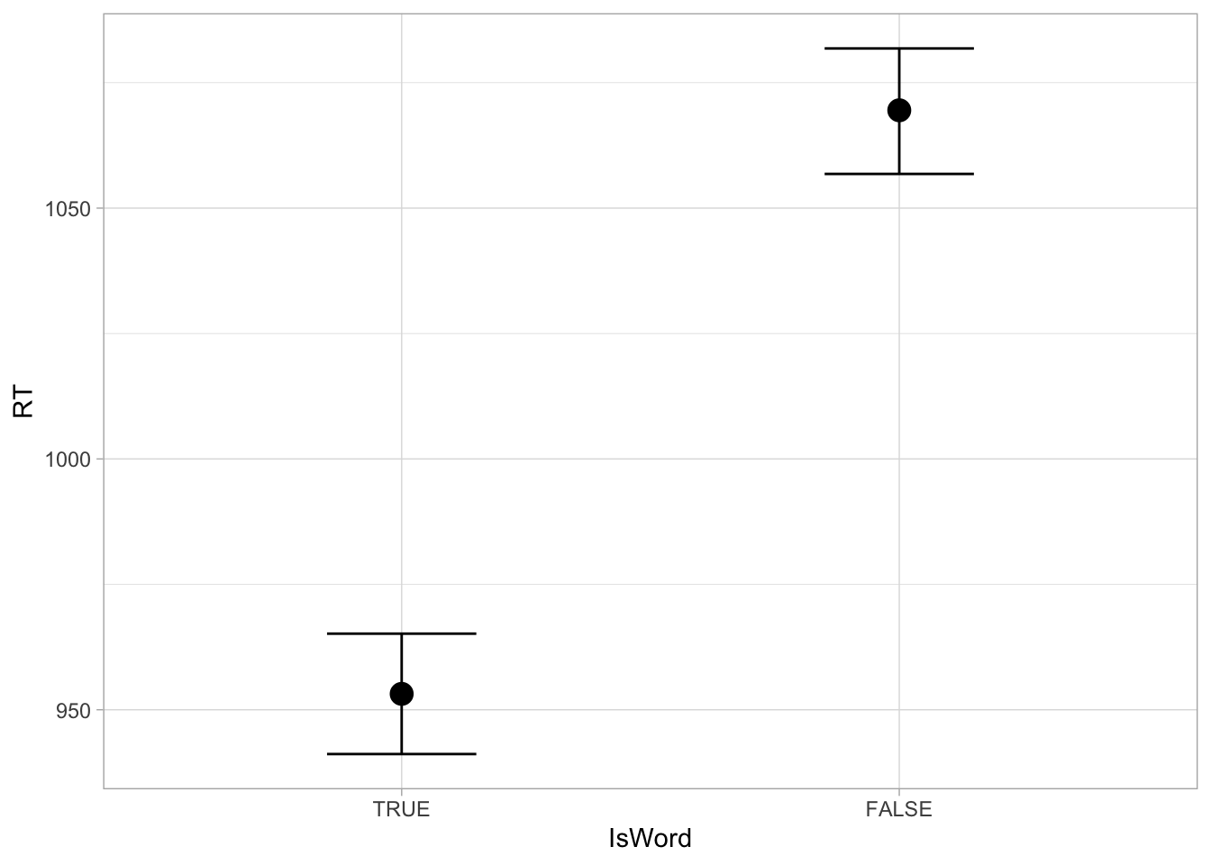
I always find plotting the full posterior distributions to be more informative (and I find the plots with error bars and dots to be potentially misleading, since they are just showing summaries of the posteriors). We already have the posterior draws of RTs with real words (b_Intercept); and those with nonce words, but to make plotting more straightforward we need to pivot the data.
Pivoting is the process of changing the shape of the data from a long format to a wide format and vice versa. You can find nice animations on Garrick Aden-Buie’s website that illustrate the process visually. What we need is pivoting from a wide to a long format: rt_bm_1_draws has two columns we are interested in, real and nonce, but to plot we need a column like word_type which says if the expected value is for real or nonce words and a column like epred for the expected prediction. We can achieve this with the pivot_longer() function from tidyr (another tidyverse package). You can learn more about pivoting in the package vignette Pivoting. We first select the two columns we want to pivot, real and nonce with select(), then we pivot with pivot_longer(): the function needs to know which columns to pivot and here we are saying to pivot all columns with the special tidyverse function everything() (note that this only works with certain tidyverse functions). Then we need to tell pivot_longer() what we want to name the column with the original column names and what name we want for the column with the values of the original columns. Check the result and play around with the code to understand how pivoting works.
rt_bm_1_long <- rt_bm_1_draws |>
  select(real, nonce) |>
  pivot_longer(everything(), names_to = "word_type", values_to = "epred")
Warning: Dropping 'draws_df' class as required metadata was removed.rt_bm_1_longNow we can plot the data with ggplot and ggdist’s stat_halfeye(). We are setting the error bars to show the 50% and 95% CrI (.width = c(0.5, 0.95)). I have also added code on the last line to manually set the “breaks” of the x-axis using the breaks argument in scale_x_continuous().
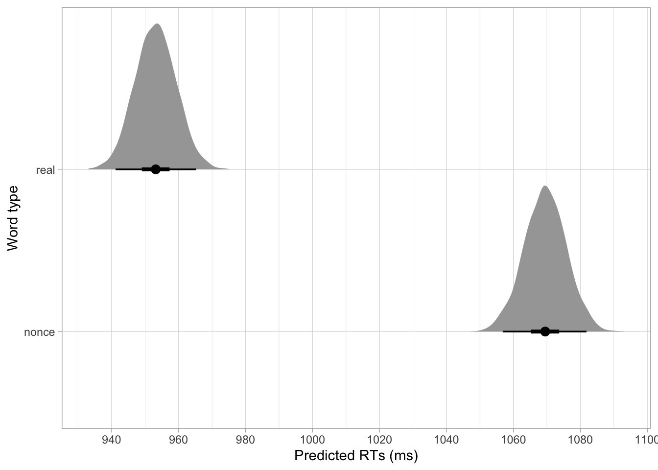
rt_bm_1_long |>
  ggplot(aes(epred, word_type)) +
  stat_halfeye(.width = c(0.5, 0.95)) +
  scale_x_continuous(breaks = seq(920, 1100, by = 20)) +
  labs(
    x = "Predicted RTs (ms)", y = "Word type"
  )
27.5 Reporting
Reporting regression models with categorical predictors is not too different from reporting models with a numeric predictor, but there are a couple of things that you need to keep in mind. With a categorical predictor you should report the estimates for the intercept, the difference from the intercept and the predicted value for the second level in the categorical predictor. You should also tell the reader how the categorical predictor was coded. Here is the full report for our model of reaction times.
We fitted a Bayesian regression model using the brms package (Bürkner 2017) in R (R Core Team 2025). We used a Gaussian distribution for the outcome variable, reaction times (in milliseconds). We included word type (real vs nonce word) as the regression predictor. Word type was coded using the default R treatment contrasts, with real word set as the reference level.
Based on the model results, there is a 95% probability that the mean RT with real words is between 941 and 965 ms (mean = 953, SD = 6). When the word is a nonce word, the RTs are between 1057 and 1082 ms at 95% confidence (mean = 1069, SD = 6). When comparing RTs for nonce vs real words, there is an 95% probability that the difference is between 99 to 134 ms (mean = 116, SD = 9). The residual standard deviation is between 306 and 319 ms (mean = 312, SD = 3).
27.6 Conclusion
To summarise, the model suggests that RTs with nonce words are 99-134 ms longer than RTs with real words. Now, is a difference of 99-134 ms a linguistically meaningful one? Statistics cannot help with that: only a well developed mathematical model of lexical retrieval and related neurocognitive processes would allow us to make any statement regarding the linguistic relevance of a particular result. This aspect applies to any statistical approach, whether frequentist or Bayesian. Within a frequentist framework (which you will learn about in Chapter 29), “statistical significance” is not “linguistic significance”. A difference between two groups can be “statistically significant” and not be linguistically meaningful and vice versa. Within the Bayesian framework, getting posterior distributions that are very certain (like the ones we have gotten so far) doesn’t necessarily mean that we have a better understanding of the processes behind the phenomenon we are investigating. After having obtained estimates from a model, always ask yourself: what do those estimates mean, based on our current understanding of the linguistic phenomenon under investigation?