In the previous chapter, I have introduced the theory behind Bayesian Gaussian models. In this chapter, you will learn how to fit Gaussian models in R. You can fit a Gaussian model to data in R using the brms package (the name is an initialism of “Bayesian Regression Models using Stan”; Gaussian models are a special type of regression models, which will be introduced in Chapter 23).
The brms package can run a variety of Bayesian (regression) models. It is a very flexible package that allows you to model a lot of different types of variables. You don’t really need to understand all of the technical details to be able to effectively use the package and interpret the results, so this textbook will focus on how to use the package in the context of research. We will cover some of the technicalities, but if you are are particularly interested in the inner workings of the package, feel free to find materials on specific aspects by searching online. One useful thing to know is that brms is a bridge between R and the statistical programming software Stan. Stan is a powerful piece of software that can run any type of Bayesian model, not just regressions. What brms does is that it allows you to write Bayesian models in R, which are translated into Stan models and run with Stan under the hood. You can safely use brms without learning Stan, but if you are interested, you can check Ch 8-10 of Nicenboim, Schad, and Vasishth (2025) and the Stan documentation.
ImportantInstallation of brms
The brms package relies on software that is external to R (the C++ toolchain) so you will have to install this extra software separately for brms to work. Following the C++ toolchain installation instructions for your operating system.
To check that the C++ installation was successful, run the following code in the RStudio Console.
library(brms)fit1 <-brm(count ~ zBase, prior =prior(normal(0, 10), class = b), data = epilepsy, chain =1)
If everything is well, you will see Compiling Stan program... and Start sampling in the console and the object fit1 should show up in the Environment tab when sampling is done.
You can run a Bayesian Gaussian model with the brm() function, short for “Bayesian Regression Model” (a Gaussian model is a special type of regression model). The mandatory arguments of brm() are a model formula, a distribution family (of the outcome variable), and the data you want to run the model with. Running a model with data is also formally known as fitting the model to the data. We want to fit a Gaussian model to reaction times from Tucker et al. (2019). Let’s revisit the mathematical formula of the model from Chapter 21 (let’s discard the priors; see the R Note box below):
\[
RT \sim Gaussian(\mu, \sigma)
\]
It would be nice if brms() allowed you to write the formula like that.
# This would be nice, but it won't work!brm( RT ~Gaussian(mu, sigma),data = mald)
Alas, due to historical and technical reasons of how other R packages write model formulae, you need to use a special way of specifying the model. As mentioned, you need three arguments: a model formula, the distribution family of the outcome, and the data. So the mathematical formula is split in two parts (corresponding to two arguments of the brm() function): formula and family.
RT ~ 1 and family = gaussian simply tell brms to model RT using a Gaussian distribution. This means that the probability distribution of the mean and the standard deviation of the Gaussian distribution of RTs will be estimated from the data. RT ~ 1 might look very weird to you right now, but it will become clear in the next couple of chapters why it is that way. For now, just accept that that is the way you write a Gaussian model in R.
We specify the data with data = mald.
As with other R functions, we want to assign the output of brm() to a variable, here rt_bm. We will then be able to inspect the output in rt_bm. Now run the Gaussian model of RTs (don’t forget to attach the brms package and read the data, like in the following code).
When you run the code, some text will be printed below the code in your Quarto document. This is what it looks like.
Compiling Stan program...Start samplingSAMPLING FOR MODEL 'anon_model'NOW (CHAIN 1).Chain 1:Chain 1: Gradient evaluation took 0.000156 secondsChain 1:1000 transitions using 10 leapfrog steps per transition would take 1.56 seconds.Chain 1: Adjust your expectations accordingly!Chain 1:Chain 1:Chain 1: Iteration:1/2000 [ 0%] (Warmup)Chain 1: Iteration:200/2000 [ 10%] (Warmup)Chain 1: Iteration:400/2000 [ 20%] (Warmup)<more text omitted>
The messages in the text are related to Stan and the statistical algorithm used by Stan to estimate the parameters of the model (in this model, these are the mean and the standard deviation of RTs). Compiling Stan program... tells you that brms has instructed Stan to compile the model specified in R and that Stan is now compiling the model to be run on the data (don’t worry if this does not make sense). Start sampling tells us that the statistical algorithm used for estimation has started. This algorithm is the Markov Chain Monte Carlo algorithm, or MCMC for short. The algorithm is run by default four times; in technical terms, four MCMC chains are run. This is why information on Chain 1, 2, 3, and 4 is printed. We will treat MCMC in more details in Chapter 25.
Now that the model has finished running and that the output has been saved in rt_bm, we can inspect it with the summary() function (note that this is different from summarise()!).
summary(rt_bm)
 Family: gaussian
  Links: mu = identity; sigma = identity
Formula: RT ~ 1
   Data: mald (Number of observations: 5000)
  Draws: 4 chains, each with iter = 2000; warmup = 1000; thin = 1;
         total post-warmup draws = 4000

Regression Coefficients:
          Estimate Est.Error l-95% CI u-95% CI Rhat Bulk_ESS Tail_ESS
Intercept  1010.50      4.45  1001.66  1019.26 1.00     3628     2476

Further Distributional Parameters:
      Estimate Est.Error l-95% CI u-95% CI Rhat Bulk_ESS Tail_ESS
sigma   317.88      3.17   311.74   324.17 1.00     4064     2571

Draws were sampled using sampling(NUTS). For each parameter, Bulk_ESS
and Tail_ESS are effective sample size measures, and Rhat is the potential
scale reduction factor on split chains (at convergence, Rhat = 1).
Let’s break down the summary bit by bit:
The first few lines are a reminder of the model we fitted:
Family is the chosen distribution for the outcome variable (RT in our model), here a Gaussian distribution.
Links lists the link functions. You don’t need to worry about these now.
Formula is the model formula.
Data reports the name of the data and the number of observations.
Finally, Draws has information about the MCMC algorithm. Again, you can discard those for now.
Then, the Regression Coefficients are listed as a table. They are called regression coefficients because brms fits Bayesian regression models and a Gaussian model is a special type of regression model (you will learn about regression models in later chapters). In the Gaussian model we fitted now, we only have one regression coefficient, Intercept, which corresponds to \(\mu\) from the formula above (for the reason why it is called that, you will have to wait until regression models are introduced in the following chapter; I apologise for the many promissory explanations…). You will learn how to interpret the Regression Coefficients table below.
The Further distributional parameters are also in the form of a table. Here we only have sigma which is \(\sigma\) from the formula above. The table has the same columns as the Regression Coefficients table.
22.1 Posterior probability distributions
The main characteristic of Bayesian models is that they don’t just provide you with a single numeric estimate for the model parameters. As mentioned in Chapter 21, the model estimates a full probability distribution for each parameter/coefficient. These probability distributions are called posterior probability distributions (or posteriors for short). They are called posterior because they are derived from the data and the prior probability distributions. The model we fitted has two parameters: the mean \(\mu\) and the standard deviation \(\sigma\). For reasons that will become clear in Chapter 23, the \(\mu\) parameter is called Intercept in the summary: you can find it in the Regression Coefficients table. The standard deviation \(\sigma\) is in the Further distributional parameters table.
TipPosterior probability distribution
A posterior probability distribution is a probability distribution of a model parameter estimated by a Bayesian model from the prior probability distribution and the data.
The Regression Coefficients table reports, for each estimated coefficient, a few summary measures of the posterior distributions of the estimated coefficients. Here, we only have the summary measures of one posterior: the posterior of the model’s mean \(\mu\). The table also has three diagnostic measures, which you can ignore for now.
Here’s a breakdown of the table’s columns:
Estimate, the mean estimate of the coefficient (i.e. the mean of the posterior distribution of the coefficient). In our model, this is the mean of the posterior distribution of the mean \(\mu\) (Intercept). Yes, you read correctly: the mean of the mean! Remember, Bayesian models estimate a full posterior probability distribution and the posterior can be summarised by a mean and a standard deviation. In this model, the posterior mean (short for mean of the posterior probability distribution) of \(\mu\) is 1010.5 ms.
Est.error, the error of the mean estimate, or estimate error. The estimate error is the standard deviation of the posterior distribution of the coefficient (here the mean \(\mu\)). Yes, the standard deviation of the mean! Again, since we are estimating a full probability distribution for \(\mu\), we can summarise it with a mean and SD as we do for any Gaussian distribution. In this model, the posterior SD of \(\mu\) is 4.45 ms. Be careful: this SD is not\(\sigma\). It is the standard deviation of the posterior distribution of the mean \(\mu\).
l-95% CI and u-95% CI, the lower and upper limits of the 95% Bayesian Credible Interval (more on these below).
Finally, Rhat, Bulk_ESS, Tail_ESS are diagnostics of the MCMC chains, which you can ignore for now.
The Further distributional parameters table has the same structure. In this model, the posterior mean of \(\sigma\) is 317.88 ms and the posterior SD of \(\sigma\) is 3.17 ms.
Putting all this together in mathematical notation:
In other words, according to the model and data, the mean or RTs is a value from the distribution \(P(1010.5, 4.45)\) and the SD of RTs is a value from the distribution \(P(317.88, 3.17)\). Here, \(P()\) stands for a generic posterior probability distribution. The model has quantified the uncertainty around the value of the \(\mu\) and \(\sigma\) parameters and this uncertainty is reflected by the fact that we get a full posterior probability distribution (summarised by its mean and SD) for each of the parameters. We don’t know exactly the values of the parameters of the Gaussian distribution assumed to have generated the sampled RTs.
ImportantR Note: Default priors in brms
One major aspect of Bayesian modelling is the combination of prior knowledge with evidence from the observed data. As introduced in Chapter 21, choosing priors is an important step in conducting Bayesian analyses. However, in this textbook we will not deal with prior specification given the quite tight schedule of the course.
If prior specification is a necessary step, how come we are not doing that? When fitting Bayesian models with brms, you are in fact using brms default priors. These are generic priors that work in most circumstances and they are equivalent to prior probability distributions that are almost flat (like in the first prior of Figure 20.1). In other words, they are so generic that they have very little influence on the posterior distribution, but still they help with the computational aspects of model fitting (which you will learn more about in Chapter 25).
If you want to inspect brms default priors, you can use the get_prior() function. Let’s do this for the model we fitted above. The function requires the model formula, the family and the data, much like the brm() function. It returns a data frame with one prior per row. The columns of interest are prior and class.
get_prior( RT ~1,family = gaussian,data = mald)
There are two priors, one for the intercept (\(\mu\)) and one for \(\sigma\) (see class column). For both \(\mu\) and \(\sigma\), brms sets a Student-t prior probability distribution. The Student-t distribution is a continuous probability distribution with three parameters: the degrees of freedom, the mean and the standard deviation. You will encounter the Student-t distribution in Chapter 29, where you will learn about frequentist p-values. For now, it will suffice to say that a Student-t distribution (also simply called a t-distribution) is similar to a Gaussian distribution (hence the two parameters, mean and SD).
Normally, you would choose priors before collecting/seeing the data. Here, brms actually uses the data to come up with generic priors that cover a wide range of values without including very unlikely values. Yet, the priors set by brms are so generic that, as said above, they bear very little effect on the posterior. So they are safe to use, even if they are based on the data itself. Just remember, thought, that if you do want to specify your own priors, you must do so independent of the data (ideally, even before you have access to the data, whether you collect it yourself or whether it is pre-existing).
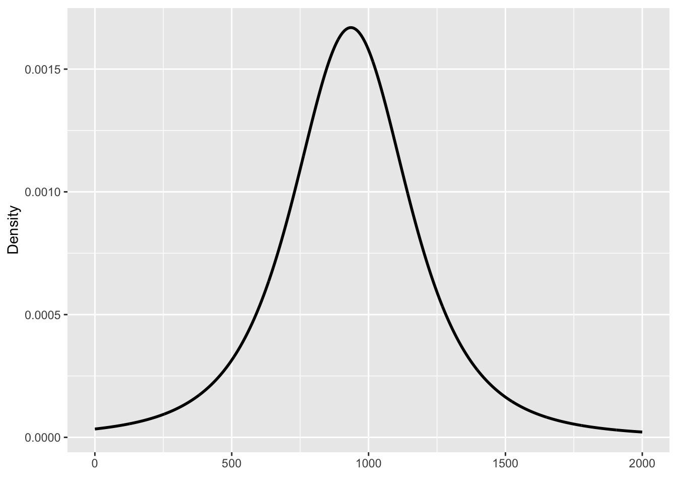
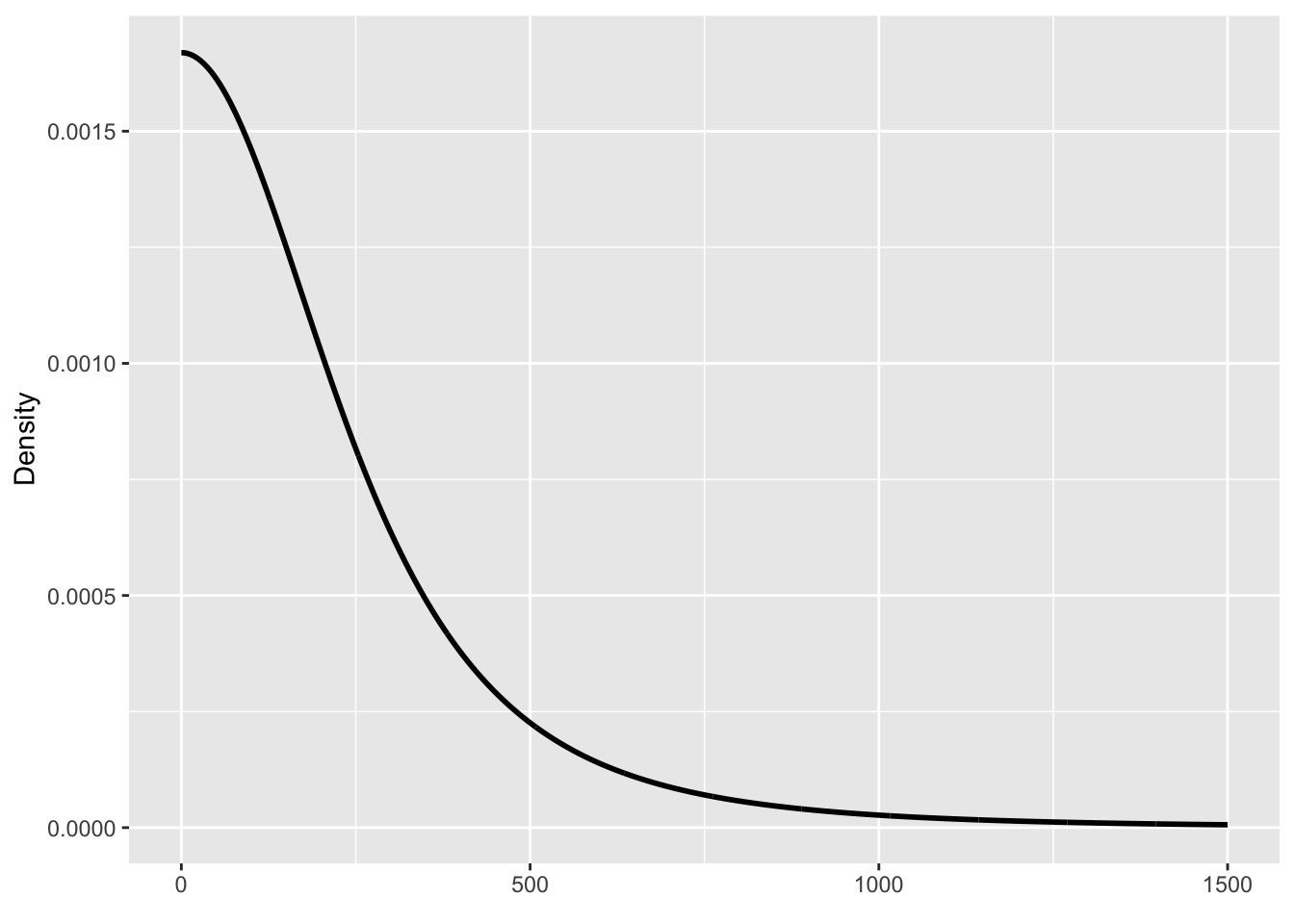
For this model and data, brms sets a t-distribution for the prior of the mean \(\mu\), with mean 935.5 and SD 220.2, and a t-distribution for the SD \(\sigma\), with mean 0 and SD 220.2. You will notice that the SDs of both priors are the same. The following figures illustrate the density curve of the priors.
x_mu <-seq(0, 2000)ggplot() +aes(x = x_mu, y = extraDistr::dlst(x_mu, 3, 935.5, 220.2)) +geom_path(linewidth =1) +labs(x =element_blank(), y ="Density" )x_sigma <-seq(0, 1500)ggplot() +aes(x = x_sigma, y = extraDistr::dlst(x_sigma, 3, 0, 220.2)) +geom_path(linewidth =1) +labs(x =element_blank(), y ="Density" )
(a) Prior probability distribution for the mean.
(b) Prior probability distribution for the SD.
Figure 22.1: Default brms priors for this chapter’s model and data.
22.2 Plotting the posterior distributions
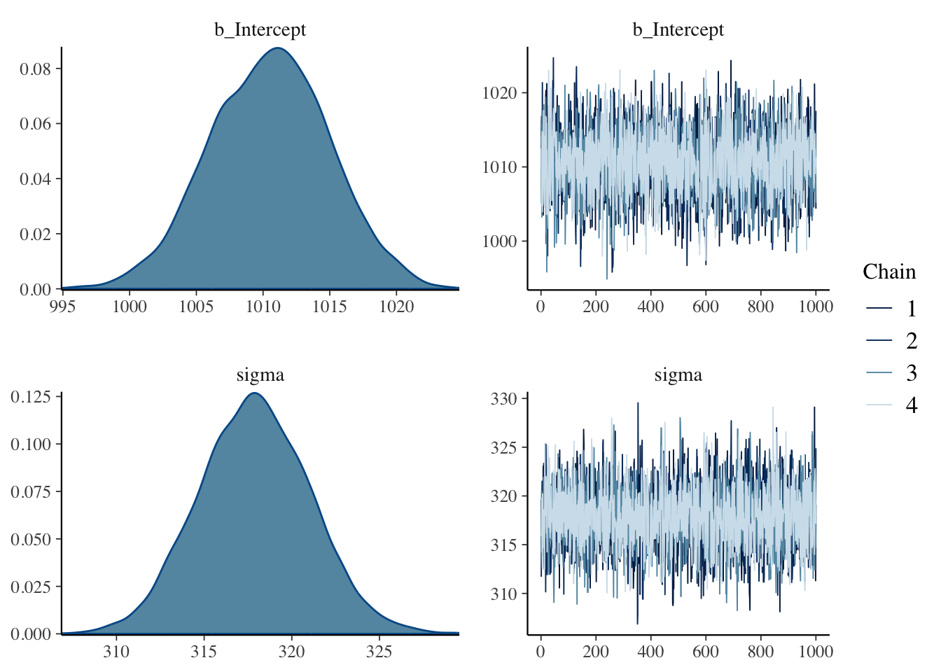
While the model summary reports summaries of the posterior distributions, it is always helpful to plot the posteriors. We can easily do so with the base R plot() function, like in Figure 22.2. The density plots of the posterior distributions of the two parameters estimated in the model are shown on the left of the figure: b_Intercept which corresponds to Intercept from the summary and sigma (the reason for why it’s b_Intercept will become clear in Chapter 23).
plot(rt_bm, combo =c("dens", "trace"))
Figure 22.2: Posterior plots of the rt_bm Gaussian model
For the b_Intercept coefficient, i.e. the mean \(\mu\), the posterior probability encompasses values between 1000 and 1020 ms, approximately. But some values are more probable than others: the values in the centre of the distribution have a higher probability density then the values on the sides. The mean of that posterior probability distribution is the Estimate value in the model summary: 1010.5 ms. Its standard deviation is the Est.error: 4.45 ms. The mean indicates the value with the highest probability density, which corresponds to the value on the horizontal axis of the density plot below the highest peak of the density curve. Based on these properties, values around 1010.5 ms are more probable than values further away from it.
For sigma, i.e. \(\sigma\), the posterior probability covers values between 310 and 325. What is the mean of the posterior probability of \(\sigma\)? The answer is in the summary, in Further distributional parameters. There you will also find the standard deviation of the posterior of \(\sigma\). That’s a standard deviation of a standard deviation! As before, this is because we are not estimating a simple value for \(\sigma\) but a full (posterior) probability distribution and we can summarise this distribution with a mean and a standard deviation. Again, the highest peak in the distribution corresponds to the Estimate value.
Now, looking at a full probability distribution like that is not very straightforward and summary measures can be even less straightforward. Credible Intervals (CrIs) help summarise the posterior distributions so that interpretation is more straightforward.
22.3 Interpreting Credible Intervals
The model summary reports the Bayesian Credible Intervals (CrIs) of the posterior distributions. Another way of returning summaries of the coefficients is to use the posterior_summary() function which returns a table (technically, a matrix, another type of R objects; we print only the first two rows with [1:2,] because we can ignore the other ones).
A Bayesian CrI is simply the central probability interval of a posterior probability distribution. You have encountered intervals in Chapter 19. By default, brms prints the 95% CrIs: these are the 95% central probability intervals of the posterior probability of each coefficient. The 95% CrI of the b_Intercept is between 1002 and 1019. This means that there is a 95% probability, or (equivalently) that we can be 95% confident, that the Intercept, i.e. \(\mu\), is within that range, given the model and data. For sigma, i.e. \(\sigma\), the 95% CrI is between 312 and 324. So, again, there is a 95% probability that the sigma value is between those values, given the model and data. So, to summarise, a 95% CrI tells us that we can be 95% confident, or in other words that there is a 95% probability, that the value of the coefficient is between the values of the CrI.
There is nothing special about 95% CrI and in fact it is recommended to calculate and report a few of them. Personally, I use 90, 80, 70 and 60% CrIs. You can get any CrI with the summary() and the posterior_summary() functions, but you will also learn an alternative and more succinct way in Chapter 24. Here is how to get an 80% CrI with summary().
summary(rt_bm, prob =0.8)
 Family: gaussian
  Links: mu = identity; sigma = identity
Formula: RT ~ 1
   Data: mald (Number of observations: 5000)
  Draws: 4 chains, each with iter = 2000; warmup = 1000; thin = 1;
         total post-warmup draws = 4000

Regression Coefficients:
          Estimate Est.Error l-80% CI u-80% CI Rhat Bulk_ESS Tail_ESS
Intercept  1010.50      4.45  1004.74  1016.14 1.00     3628     2476

Further Distributional Parameters:
      Estimate Est.Error l-80% CI u-80% CI Rhat Bulk_ESS Tail_ESS
sigma   317.88      3.17   313.84   321.89 1.00     4064     2571

Draws were sampled using sampling(NUTS). For each parameter, Bulk_ESS
and Tail_ESS are effective sample size measures, and Rhat is the potential
scale reduction factor on split chains (at convergence, Rhat = 1).
For posterior_summary(), you specify the percentiles rather than the probability level.
Here you have the results from the regression model. Really, the results of the model are the full posterior probabilities, but it makes things easier to focus on the CrIs. If you are used to frequentist statistics (either from learning how to run them or from reading frequentist analyses in academic papers) this might seem a bit underwhelming. But this is the core thinking of Bayesian statistics: inference is based on full probability distributions for the model’s parameters, rather than on a single value (like a p-value).
22.4 Reporting
What about reporting the model in writing? We could report the model and the results like this (for simplicity, we report only the 95% CrIs here. You will learn how to report multiple CrIs in tables later).1
We fitted a Bayesian Gaussian model of reaction times (RTs) using the brms package (Bürkner 2017) in R (R Core Team 2024). The model estimates the mean and standard deviation of RTs.
Based on the model results, there is a 95% probability that the mean is between 1002 and 1019 ms (mean = 1011, SD = 4) and that the standard deviation is between 312 and 324 ms (mean = 318, SD = 3).
The example used in this chapter is quite trivial: we are just estimating a mean and SD from the data, but in order to understand how to answer more involved questions it is fundamental that you understand what was covered in this chapter. So make sure you have grasped the basics of Gaussian models before moving onto regressions in Chapter 23. On the other hand, if you are ever asked what we can expect RTs in an auditory lexical decision task to look like you might be able to say that, based on the model and data in this chapter, we can be quite confident that they will have a mean of about 1010 ms and an SD of about 320 ms. You might think this was a lot of work to just learn about what we knew directly from the sample, and it is, but be reassured that in normal research contexts things are always much more complex than this, so it is indeed worth the effort.
NoteQuiz 1
Which function is used to fit Bayesian models?
The Estimate column in further distributional parameters is:
The posterior of each parameter is the value in the Estimate column.
Only 95% CrI should be used for inference.
To fit a Gaussian model, the formula has the form y ~ 1.
The intercept corresponds to the parameter \(\mu\).
Nicenboim, Bruno, Daniel J. Schad, and Shravan Vasishth. 2025. Introduction to Bayesian Data Analysis for Cognitive Science. https://bruno.nicenboim.me/bayescogsci/.
Tucker, Benjamin V, Daniel Brenner, Kyle Danielson D, Matthew C Kelley, Filip Nenadić, and Michelle Sims. 2019. “The Massive Auditory Lexical Decision (MALD) Database.”Behavior Research Methods 51 (3): 11871204. https://doi.org/10.3758/s13428-018-1056-1.
To know how to add a citation for any R package, simply run citation("package") in the R Console, where "package" is the package name between double quotes.↩︎