20 Bayesian inference

In Chapter 18 and Chapter 19 you learned about probabilities, probability distributions and probability intervals. Statistical inference (Chapter 6) is built on probability, but, while probabilities and distributions are precise mathematical concepts, their more philosophical interpretation varies depending on which stance one adopts. Among the two most common approaches to interpreting probability there are the frequentist and the Bayesian approach. Most of current research is carried out with frequentist methods. This is a historical accident, based on both an initial misunderstanding of Bayesian statistics (which is, by the way, older than frequentist statistics) and the fact that frequentist maths was much easier to work with (and personal computers did not exist). Despite the wide-spread use of frequentist statistics, this textbook (and related course) teaches you statistics in the Bayesian approach. There are several reasons for preferring Bayesian over frequentist statistics, both from a pedagogical and practical perspective, but until you learn more about frequentist statistics in Chapter 29, you will have to trust us for now.

Probabilities in a frequentist framework are about average occurrences of events in a hypothetical series of repetitions of those events. Imagine you observe a volcano for a long period of time. The number of times the volcano erupts within that time tells us the frequency of occurrence of the event of volcanic eruption. In other words, it tells us its (frequentist) probability. In the Bayesian framework, probabilities are about the level of (un)certainty that an event will occur at any specific time given certain conditions. This is probably the way we normally think about probabilities: like in the weather forecast, if somebody tells you tomorrow it will rain with a probability of 85%, you intuitively know that it is very likely that it will rain tomorrow although it is not certain. In the context of research, a frequentist probability tells you the probability of obtaining the same result again and again given an imaginary series of replications of the study that generated that probability. On the other hand, a Bayesian probability tells you the probability of your hypothesis given the results of your study and your prior beliefs.

Bayesian inference approaches are now gaining momentum in many fields, including linguistics. The main advantage of Bayesian inference is that it allows researchers to answer research questions in a more straightforward way, using a more intuitive take on uncertainty and probability than what frequentist methods can offer. Bayesian inference is based on the concept of updating prior beliefs in light of new data. Given a set of prior probabilities and observations, Bayesian inference allows us to revise those prior probabilities and produce posterior probabilities. This is possible through the Bayesian interpretation of probabilities in the context of Bayes’ Theorem, which takes the name from Rev. Thomas Bayes (1701–1771).

In simple conceptual terms, the Bayesian interpretation of Bayes’ Theorem states that the probability of a hypothesis \(h\) given the observed data \(d\) is proportional to the product of the prior probability of \(h\) and the probability of \(d\) given \(h\).

\[ P(h|d) \sim P(h) \cdot P(d|h) \]

The prior probability \(P(h)\) represents the researcher’s beliefs towards \(h\). These beliefs can be based on expert knowledge, previous studies or mathematical principles.

Let’s see a practical example of Bayesian updating based on the “globe-tossing” scenario described in McElreath (2020), Ch 2 (originally from Gelman, Nolan, and Nolan (2011)). Imagine holding a small globe that represents Earth. You want to know what fraction of its surface is covered by water. To estimate this, you adopt a simple method: toss the globe into the air, and when you catch it, note whether the spot under your right index finger is water (W) or land (L). Then toss it again and repeat. This process produces a sequence of observations. For example, the first nine outcomes might be: WLWWWLWLW. In this sequence, six outcomes are water and three are land. We call this sequence the data, i.e. \(d\). What we are trying to estimate here is the true proportion of water.

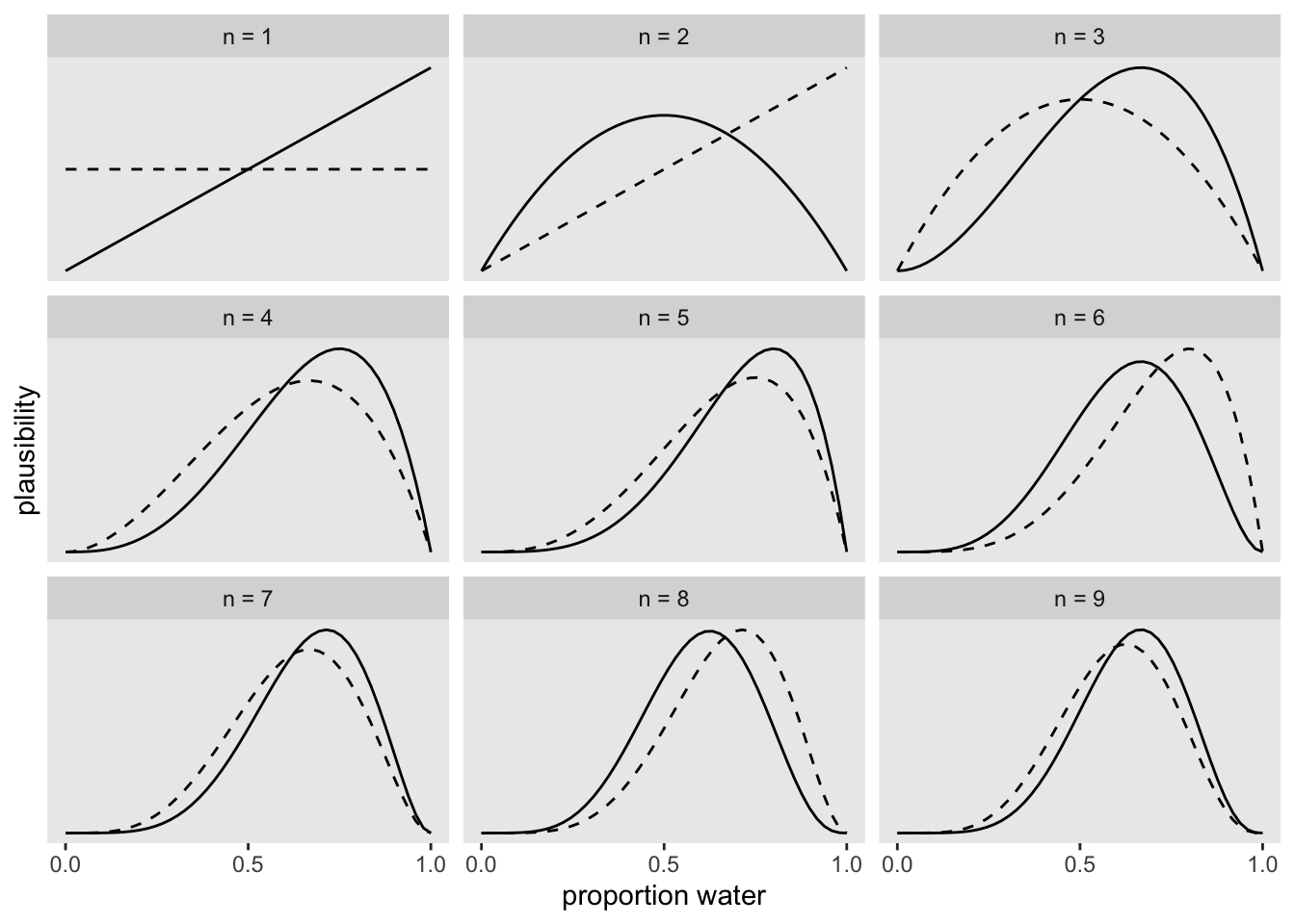
So what about our prior beliefs about the true proportion of water, i.e. \(P(h)\)? Let’s say that our prior belief (assuming complete ignorance about the true proportion of water) is that all proportions are equally probable. This is called a uniform prior, or a flat prior. You can see why in Figure 20.1. If you look at the top-right panel (the one with “n = 1”), the dashed line represents our prior belief: all proportions of water (on the x-axis) are equally probable, so that the prior probability distribution is flat. Note that a probability of 0 means Earth is all land, and a probability of 1 means Earth is all water. Now, let’s update the flat prior distribution with the first observation in the globe-tossing exercise: the first outcome was W, water. This observations corresponds to a distribution in which 1 has the greatest probability and values below it have decreasing probability. This is represented in the top-right panel of Figure 20.1 as the solid slanted line. This is \(P(d | h)\). If we combine the flat prior and the probability of the data we get the dashed line in the second top panel (with “n = 2”). That is the posterior probability distribution resulting from the Bayesian update at step “n = 1”. This becomes the prior probability distribution at step “n = 2”.

Code

# Code adapted from: https://bookdown.org/content/4857/small-worlds-and-large-worlds.html#bayesian-updating.

sequence_length <- 50

d <- tibble(toss = c("w", "l", "w", "w", "w", "l", "w", "l", "w")) |> 
  mutate(n_trials  = 1:9,
         n_success = cumsum(toss == "w"))

d |> 
  expand_grid(p_water = seq(from = 0, to = 1, length.out = sequence_length)) |> 
  group_by(p_water) |> 
  # to learn more about lagging, go to:
  # https://www.rdocumentation.org/packages/stats/versions/3.6.2/topics/lag
  # https://dplyr.tidyverse.org/reference/lead-lag.html
  mutate(lagged_n_trials  = lag(n_trials),
         lagged_n_success = lag(n_success)) |> 
  ungroup() |> 
  mutate(prior      = ifelse(n_trials == 1, .5,
                             dbinom(x    = lagged_n_success, 
                                    size = lagged_n_trials, 
                                    prob = p_water)),
         likelihood = dbinom(x    = n_success, 
                             size = n_trials, 
                             prob = p_water),
         strip      = str_c("n = ", n_trials)) |> 
  # the next three lines allow us to normalize the prior and the likelihood, 
  # putting them both in a probability metric 
  group_by(n_trials) |> 
  mutate(prior      = prior / sum(prior),
         likelihood = likelihood / sum(likelihood)) |>   
  
  # plot!
  ggplot(aes(x = p_water)) +
  geom_line(aes(y = prior), 
            linetype = 2) +
  geom_line(aes(y = likelihood)) +
  scale_x_continuous("proportion water", breaks = c(0, .5, 1)) +
  scale_y_continuous("plausibility", breaks = NULL) +
  theme(panel.grid = element_blank()) +
  facet_wrap(~ strip, scales = "free_y")

Figure 20.1: Bayesian updating of a prior based on observations. From McElreath (2020) and Kurtz (2023).

Now let’s update our latest prior with the probability taken from the second observation: this was L, land. The solid line in the second panel is the probability of getting a W and L: the probability indicates that a proportion of 0.5 is the most probable. This makes sense: if in two tosses you got one W and one L, then the most probable hypothesis is that there is 50% of water and 50% of land. We combine again our prior (dashed line) with the data (solid line) to obtain the dashed line in the third top panel. This is our new prior. The rest of the figure shows how the prior gets updated at each new observation of W or L. You see that the highest density of the dashed lines quickly moves to the right. They are now suggesting that the globe has a higher proportion of water than land. Chapter 2 of McElreath (2020) goes into much more details and I recommend you read that at some point if you feel this section felt a bit too abstract.

Hopefully you can appreciate how different the frequentist and Bayesian approaches are: while frequentist statistics focusses on the rejection of a null/nil hypothesis based on the probability of the data given the hypothesis, or \(P(d|h)\), Bayesian statistics is about obtaining the probability of any hypothesis given the data, or \(P(h|d)\). You might also realise now that \(P(d|h)\) appears in Bayes’ Theorem. But the theorem also includes the prior, \(P(h)\). This is totally missing in the frequentist approach.