Code
library(tidyverse)

line <- tibble(
  x = c(2, 4, 5, 8, 10, 23, 36),
  y = 3 + 2 * x
)

ggplot(line, aes(x, y)) +
  geom_point(size = 4) +
  geom_line(colour = "red") +
  labs(title = bquote(italic(y) == 3 + 2 * italic(x)))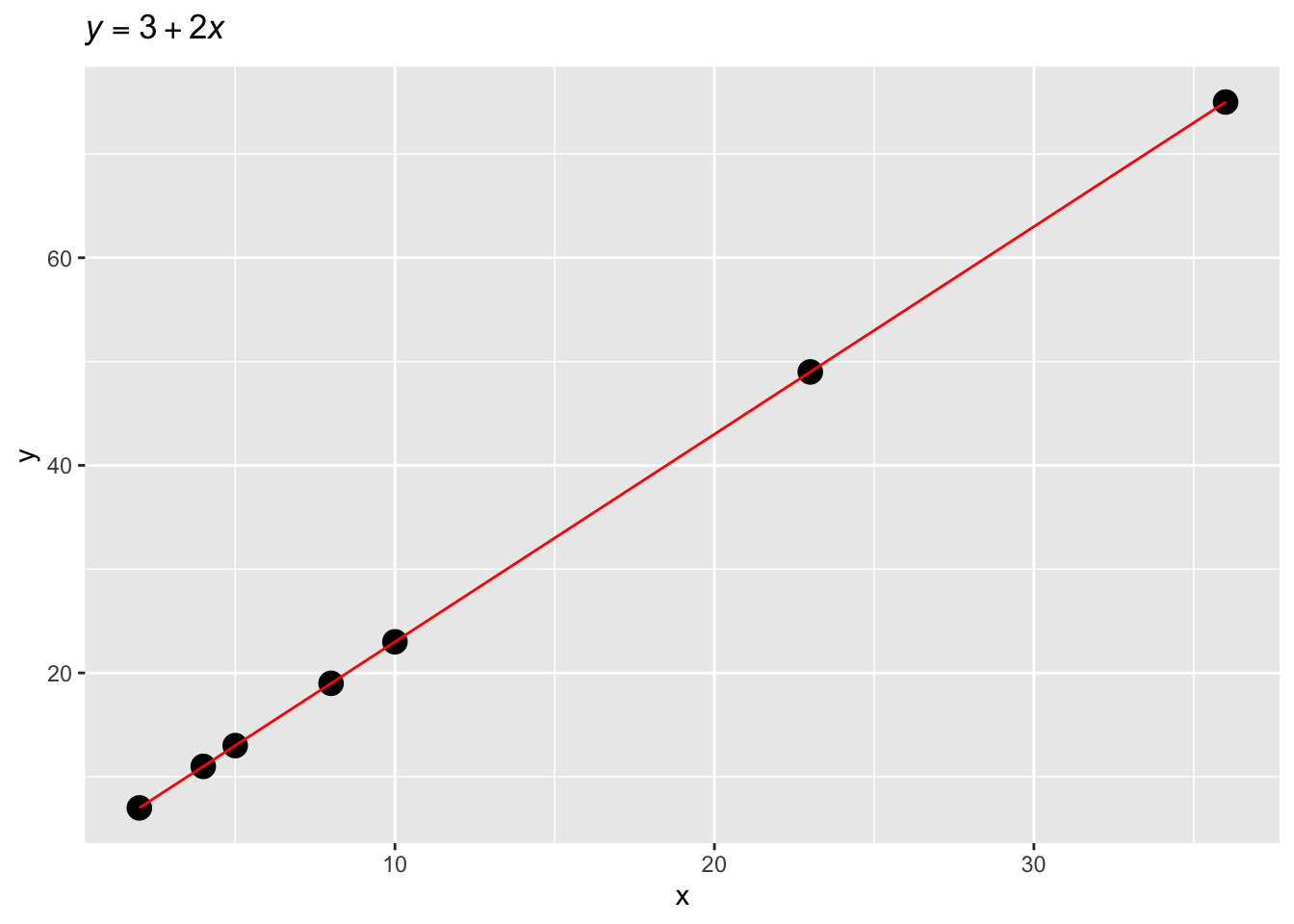
![]()
In the previous chapters, you have learned the basics of probability and how to run Gaussian models to estimate the mean and standard deviation (\(\mu\) and \(\sigma\)) of a variable. This chapter extends the Gaussian model to what is commonly called a Gaussian regression model (or simply regression model). Regression models (including the Gaussian) are models based on the equation of a straight line. This is why regression models are also called linear models. Regression models allow you to model the relationship between two or more variables. This textbook introduces you to regression models of increasing complexity which can model variables frequently encountered in linguistics. Note that regression models are very powerful and flexible statistical models which can deal with a great variety of types of variables. Appendix B has a regression cheat sheet which you will be able to consult, after completing this course, as a guide for building a regression model based on a set of questions. For now, let’s dive into the basics of a regression model.
A regression model is a statistical model that estimates the relationship between an outcome variable and one or more predictor variables (more on outcome/predictor below). Regression models are based on the equation of a straight line.
\[ y = mx + c \]
An alternative notation of the equation is:
\[ y = \beta_0 + \beta_1 x \]
\(\beta\) is the Greek letter beta [ˈbiːtə]: you can read \(\beta_0\) as “beta zero” and \(\beta_1\) “beta one”. In this formula, \(\beta_0\) corresponds to \(c\) and \(\beta_1\) to \(m\) in the first notation. We will use the second notation (with \(\beta_0\) and \(\beta_1\)) in this book, since using \(\beta\)’s with subscript indexes will help understand the process of extracting information from regression models later.1
You might remember from school when you were asked to find the values of \(y\) given certain values of \(x\) and specific values of \(\beta_0\) and \(\beta_1\). For example, you were given the following formula (the dot \(\cdot\) stands for multiplication; it can be dropped so \(2 \cdot x\) and \(2x\) are equivalent):
\[ y = 3 + 2 \cdot x \]
and the values \(x = (2, 4, 5, 8, 10, 23, 36)\). The homework was to calculate the values of \(y\) and maybe plot them on a Cartesian coordinate space.
library(tidyverse)
line <- tibble(
x = c(2, 4, 5, 8, 10, 23, 36),
y = 3 + 2 * x
)
ggplot(line, aes(x, y)) +
geom_point(size = 4) +
geom_line(colour = "red") +
labs(title = bquote(italic(y) == 3 + 2 * italic(x)))
Using the provided formula, we are able to find the values of \(y\). Note that in \(y = 3 + 2 * x\), \(\beta_0 = 3\) and \(\beta_1 = 2\). Importantly, \(\beta_0\) is the value of \(y\) when \(x = 0\). \(\beta_0\) is commonly called the intercept of the line. The intercept is the value where the line crosses the y-axis (the value where the line “intercepts” the y-axis).
\[ \begin{aligned} y & = 3 + 2 x\\ & = 3 + 2 \cdot 0\\ & = 3\\ \end{aligned} \]
And \(\beta_1\) is the number to add to the intercept for each unit increase of \(x\). \(\beta_1\) is commonly called the slope of the line.2 Figure 23.1 should clarify this. The dashed line indicates the increase in \(y\) for every unit increase of \(x\) (i.e., every time \(x\) increases by 1, \(y\) increases by 2).
line <- tibble(
  x = 0:3,
  y = 3 + 2 * x
)

ggplot(line, aes(x, y)) +
  geom_point(size = 4) +
  geom_line(colour = "red") +
  annotate("path", x = c(0, 0, 1), y = c(3, 5, 5), linetype = "dashed") +
  annotate("path", x = c(1, 1, 2), y = c(5, 7, 7), linetype = "dashed") +
  annotate("path", x = c(2, 2, 3), y = c(7, 9, 9), linetype = "dashed") +
  annotate("text", x = 0.25, y = 4.25, label = "+2") +
  annotate("text", x = 1.25, y = 6.25, label = "+2") +
  annotate("text", x = 2.25, y = 8.25, label = "+2") +
  scale_y_continuous(breaks = 0:15) +
  labs(title = bquote(italic(y) == 3 + 2 * italic(x)))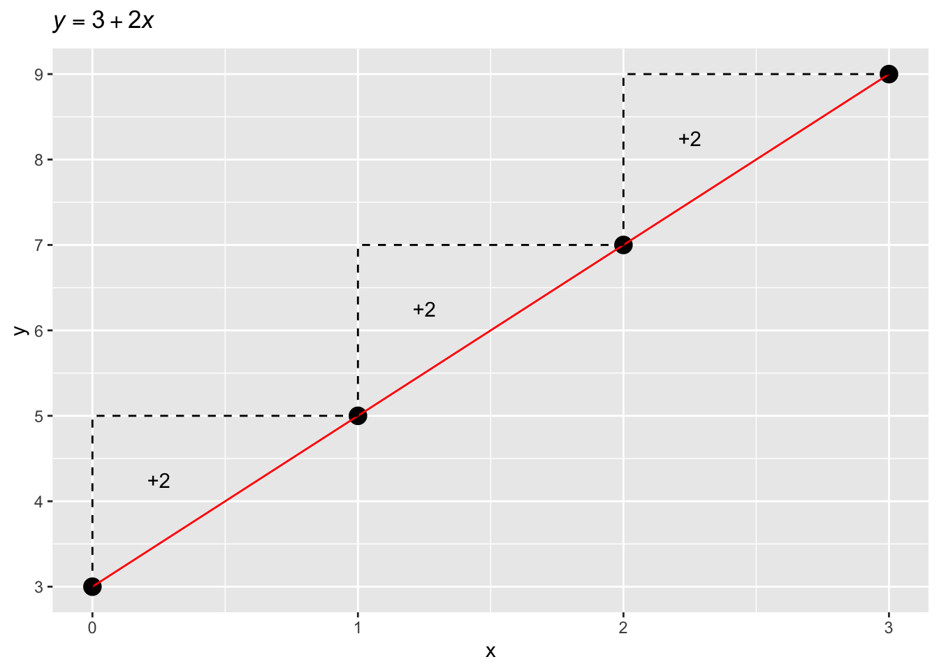
Of course, we can plug in any value of \(x\) in the formula to obtain \(y\). The following equations show \(y\) when \(x\) is 1, 2, and 3. You see that when you go from \(x = 1\) to \(x = 2\) we go from \(y = 5\) to \(y = 7\): \(7 - 5 =2\), our slope \(\beta_1\).
\[ \begin{aligned} y & = 3 + 2 \cdot 1\\ & = 3 + 2\\ & = 5\\ y & = 3 + 2 \cdot 2\\ & = 3 + 4\\ & = 7\\ y & = 3 + 2 \cdot 3\\ & = 3 + 6\\ & = 9\\ \end{aligned} \]
Now, in the context of research, you usually start with a sample of measures (values) of \(x\) (the predictor variable) and \(y\) (the outcome variable), rather than having to calculate \(y\). Then you have to estimate (i.e. to find the values of) \(\beta_0\) and \(\beta_1\) of the model formula \(y = \beta_0 + \beta_1 x\) . This is what regression models are for: given the sampled values of \(y\) and \(x\), the model estimates \(\beta_0\) and \(\beta_1\).
Measurements are noisy: they usually contain errors. Error can have many different causes (for example, measurement error due to technical limitations or variability in human behaviour), but we are usually not that interested in learning about what causes the error. Rather, we just want our model to be able to deal with error. Let’s see what errors looks like. Figure 23.2 shows values of \(y\) simulated with the equation \(y = 1 + 1.5x\) (with \(x\) equal 1 to 10), to which the random error \(\epsilon\) (the Greek letter epsilon [ˈɛpsɪlɒn]) was added. Due to the added error, the points are almost on the straight line defined by \(y = 1 + 1.5x\), but not quite. The vertical distance between the observed points and the expected line, called the regression line, is the residual error (red lines in the plot).
set.seed(4321)
x <- 1:10
y <- (1 + 1.5 * x) + rnorm(10, 0, 2)

line <- tibble(
  x = x,
  y = y
)

m <- lm(y ~ x)
yhat <- m$fitted.values
diff <- y - yhat
ggplot(line, aes(x, y)) +
  geom_segment(aes(x = x, xend = x, y = y, yend = yhat), colour = "red") +
  geom_point(size = 4) +
  geom_smooth(method = "lm", formula = y ~ x, se = FALSE) +
  scale_x_continuous(breaks = 1:10) +
  labs(title = bquote(italic(y) == 1 + 1.5 * italic(x) + epsilon))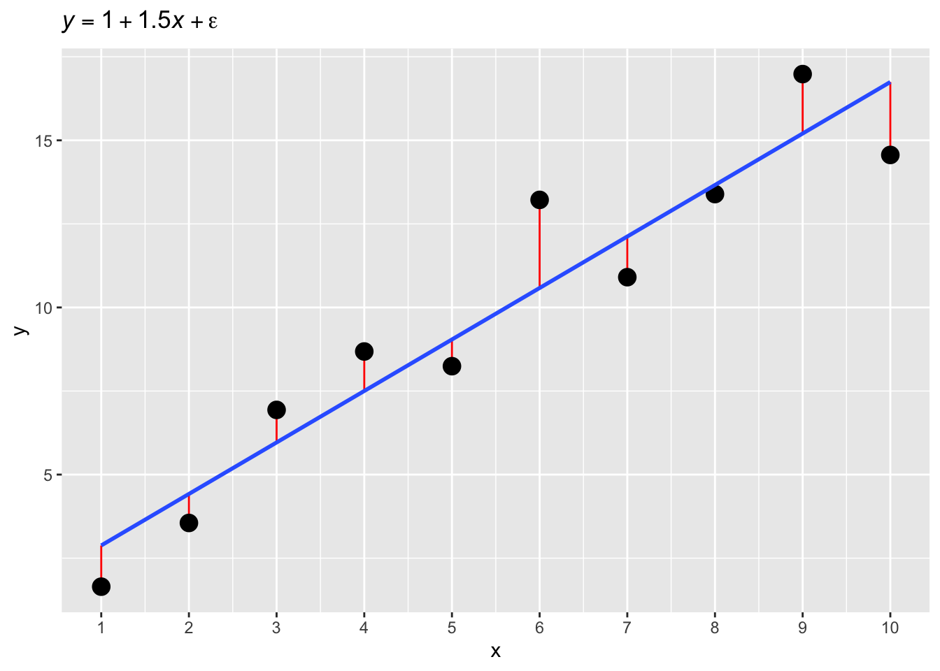
When taking into account error, the equation of a regression model becomes the following:
\[ y = \beta_0 + \beta_1 x + \epsilon \]
where \(\epsilon\) is the error. In other words, \(y\) is the sum of \(\beta_0\), \(\beta_1 x\) and some error. In regression modelling, the error \(\epsilon\) is assumed to come from a Gaussian distribution with mean 0 and standard deviation \(\sigma\) when \(y\) is assumed to be generated by a Gaussian distribution: \(\epsilon \sim Gaussian(\mu = 0, \sigma)\). We can substitute \(\epsilon\) for the distribution.
\[ y = \beta_0 + \beta_1 x + Gaussian(0, \sigma) \]
Furthermore, this equation can be rewritten like so (since the mean of the Gaussian error is 0):
\[ \begin{aligned} y & \sim Gaussian(\mu, \sigma)\\ \mu & = \beta_0 + \beta_1 x\\ \end{aligned} \]
You can read those formulae like so: “The variable \(y\) is distributed according to a Gaussian distribution with mean \(\mu\) and standard deviation \(\sigma\). The mean \(\mu\) is equal to the intercept \(\beta_0\) plus the slope \(\beta_1\) times the variable \(x\).” This is a Gaussian regression model, because the assumed family of the outcome \(y\) is Gaussian. Now, the goal of a (Gaussian) regression model is to estimate \(\beta_0\), \(\beta_1\) and \(\sigma\) from the data (i.e. from the values of \(x\) and \(y\)). In other words, regression models find the regression line based on the observations of \(y\) and \(x\). We do not know what is the true regression line that has generated \(y\) and \(x\), we just have \(y\) and \(x\) values.
The \(y \sim Gaussian(\mu, \sigma)\) line in the formulae above is exactly the formula you saw in Chapter 21. It is no coincidence: this is Gaussian regression model. The outcome variable \(y\) is assumed to be Gaussian. The new building block we have added now is that \(\mu\) depends on \(x\): this is because \(x\) appears in the formula of \(\mu\). In other words, we are allowing the mean \(\mu\) to vary with \(x\). This is expressed by the so-called regression equation (also linear equation): \(\mu = \beta_0 + \beta_1 x\). This is the core concept of regression models.
You perhaps realised this by now, but the regression equation implies that both \(y\) and \(x\) are numeric variables. However, regression models can also be used with variables that are categorical. You will learn how to use categorical predictors (categorical \(x\)’s) in regression models in Week 7’s chapters. Moreover, regression models are not limited to the Gaussian distribution family and in fact regression models can be fit with virtually any other distribution family. The chapters of Week 8 will teach you how to fit two other useful distribution families: the log-normal family and the Bernoulli family. You will be able to learn about other families by checking the resources linked in Appendix B.
Galton and regression
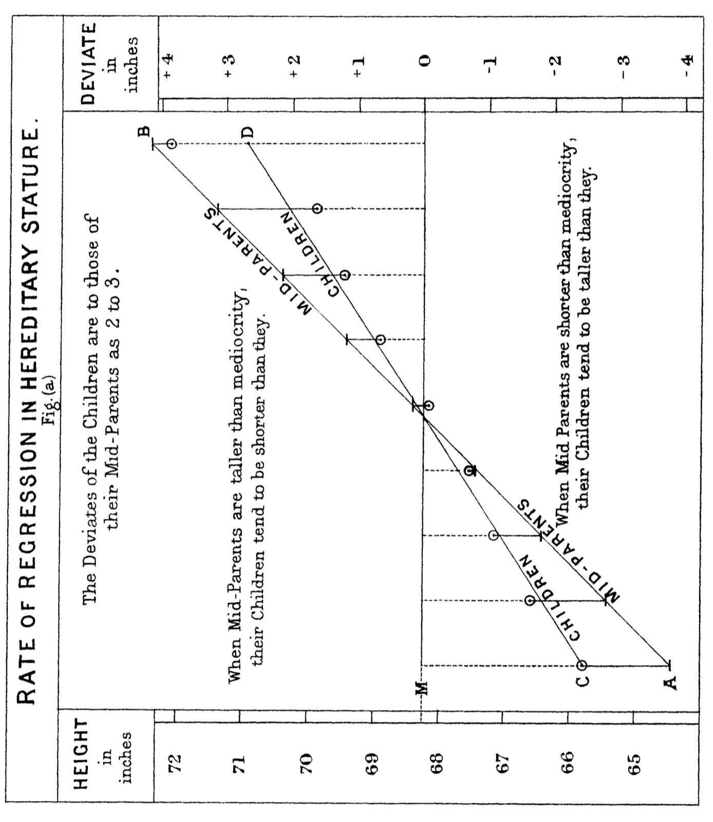
The basic logic of regression models is attributed to Francis Galton (1822–1911). Galton studied the relationship between the heights of parents and their children (Galton 1980, 1886). He noticed that while tall parents tended to have tall children, the children’s heights were often closer to the average height of the population. This phenomenon, which he called “regression toward mediocrity” (now known as “regression to the mean”), showed that extreme values (e.g., very tall or very short parents) were less likely to be perfectly transmitted to the next generation.
The core idea of Galton’s framework can be expressed as a regression model:
\[ y = \beta_0 + \beta_1 \cdot x + \epsilon \]
where:
Galton found that the slope \(\beta_1\) was less than 1, meaning that the children’s heights were not as extreme as their parents’ heights. For example, if tall parents (above the mean) had an average child height increase of \(\beta_1 < 1\), it indicated a “regression” toward the population mean. The intercept \(\beta_0\) ensured the line passed through the mean of both parents’ and children’s heights.
Galton, eugenics and racism
Galton is considered one of the founders of modern statistics and is widely recognized for his contributions to fields such as regression, correlation, and the study of heredity. However, his work is also deeply intertwined with controversial and now discredited views on race and eugenics. Galton coined the term eugenics in 1883, defining it as the “science of improving the genetic quality of the human population”. His goal was to encourage the reproduction of individuals he deemed “fit” and discourage that of those he considered “unfit”. He promoted selective breeding among humans, drawing inspiration from animal breeding practices.
Galton believed in a hierarchy of intelligence and ability among “races”, a belief that was common among many European intellectuals of his time. In works like Hereditary Genius (1869), he argued that intelligence and other traits were hereditary and that Europeans were superior to other racial groups. These conclusions were based on flawed assumptions and biased interpretations of data. His ideas contributed to the spread of pseudo-scientific racism, which attempted to justify inequality and colonialism.
Galton’s eugenic ideas were later used to justify discriminatory policies, including forced sterilization programs and racial segregation in various countries. While Galton himself did not directly advocate for many of the extreme measures implemented in the 20th century, his work laid the groundwork for such abuses. His promotion of eugenics and racial hierarchies has left a damaging legacy.