polite <- read_csv("data/winter2012/polite.csv")
polite34 Regression models: multiple predictors
![]()
![]()
So far, we fitted regressions with a single predictor, like the following Gaussian model of reaction times from Chapter 27 using the data from Tucker et al. (2019):
\[ \begin{aligned} RT_i & \sim Gaussian(\mu_i, \sigma)\\ \mu_i & = \beta_0 + \beta_1 \cdot w_i\\ \end{aligned} \]
The categorical predictor \(W\) (IsWord in the data) has two levels (TRUE and FALSE), so there is one intercept and one coefficient for the dummy variable \(w_i\): \(\beta_0\) and \(\beta_1\). In most context, however, you will want to investigate the effects of more than one predictor. Regression models can be fit with multiple predictors. Traditionally, regression models with a single predictor were called “simple regression” and models with more than one “multiple regression”, but it doesn’t make sense to have a specific name: they are all regression models. In this chapter, we will discuss regression models with two categorical predictors.
34.1 Two categorical predictors
To illustrate how to fit and interpret models with two categorical predictors, we will use the winter2012/polite.csv data from Winter and Grawunder (2012). The data contains several acoustic measures from the speech of Korean speakers. The participants of the study were asked to make a request imagining they were speaking either to a friend or to someone of higher status, thus producing speech in both an informal and polite condition, respectively. This is coded in the attitude column of the polite data, which we read in the code below.
The polite data also contains information about the gender of the participant: in the data there are female and male participants. In this chapter we will model the mean fundamental frequency (f0) of each utterance depending on gender and attitude. The data contains some missing f0 data, so we filter it out first.
polite_filt <- polite |>
  drop_na(f0mn)
Now let’s plot mean f0 by gender and attitude. We can achieve this by using a jitter plot by gender, with coloured points by attitude. Figure 34.1 shows this plot. However, the plot is not very legible because the points for informal and polite attitude are on the same vertical axis.
polite_filt |>
  ggplot(aes(gender, f0mn, colour = attitude)) +
  geom_jitter()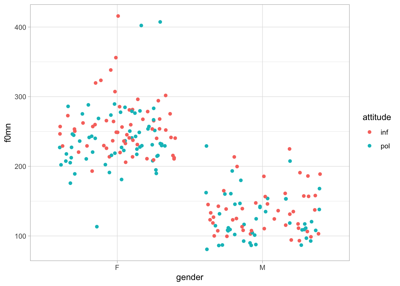
We can improve the plot by “dodging” the jitter for informal and polite attitude with the position argument in geom_jitter(). The argument takes one of the position functions: here we want position_jitterdodge(), used to dodge the jitter geometry. The dodge.width argument sets how far apart the jitters should be (the width of the dodging). Figure 34.2 is clearer, now that the jitters are dodged.
polite_filt |>
  ggplot(aes(gender, f0mn, colour = attitude)) +
  geom_jitter(position = position_jitterdodge(dodge.width = 1))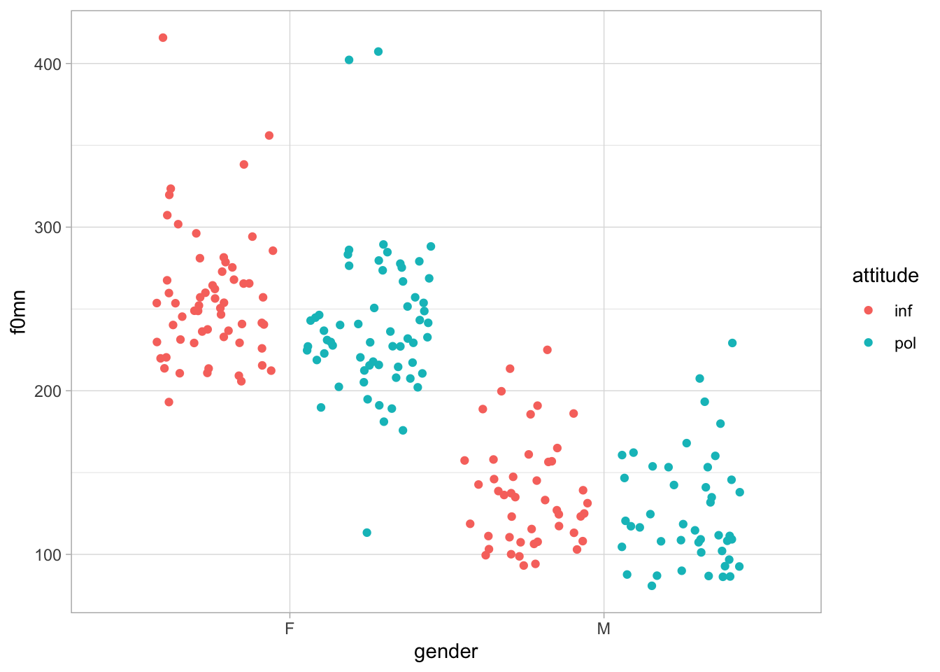
34.2 Fitting the model
We can now move onto fitting a regression model to f0mn, with gender and attitude as two categorical predictors. Here is what the model formula would look like:
\[ \begin{aligned} f0mn_i & \sim Gaussian(\mu_i, \sigma) \\ \mu_i & = \beta_0 + \beta_1 \cdot gen_{\text{M}[i]} + \beta_2 \cdot att_{\text{POL}[i]} \end{aligned} \]
The formula has two indicator variables: \(gen_{\text{M}}\) and \(att_{\text{POL}}\). The first variable states if the \(f0mn\) value is from a female participant (\(gen_{\text{M}} = 0\)) or a male participant (\(gen_{\text{M}} = 1\)). The second variable states if the \(f0mn\) value is from the informal condition (\(att_{\text{POL}} = 0\)) or the polite condition (\(att_{\text{POL}} = 1\)). Table 34.1 shows the treatment contrasts table.
| \(gen_\text{M}\) | \(att_\text{POL}\) | |
|---|---|---|
gender = F and attitude = informal |
0 | 0 |
gender = F and attitude = polite |
0 | 1 |
gender = M and attitude = informal |
1 | 0 |
gender = M and attitude = polite |
1 | 1 |
Fitting a regression model with multiple predictors is as easy as just adding the predictors in the formula using a +: f0mn ~ gender + attitude. Note that from this point on we won’t include the 1 + any more, since it’s implicit, but you can still write it out if you wish. The rest of the code has no surprises.
f0_bm <- brm(
  f0mn ~ gender + attitude,
  family = gaussian,
  data = polite,
  cores = 4,
  seed = 7123,
  file = "cache/ch-regression-cat-cat_f0_bm"
)
34.3 Interpreting models with multiple categorical predictors
Let’s print out the model summary. If you look at the Regression Coefficients table, you will find three coefficients, each matching one of the \(\beta\) coefficients in the \(\mu\) formula above.
summary(f0_bm) Family: gaussian
Links: mu = identity; sigma = identity
Formula: f0mn ~ gender + attitude
Data: polite (Number of observations: 212)
Draws: 4 chains, each with iter = 2000; warmup = 1000; thin = 1;
total post-warmup draws = 4000
Regression Coefficients:
Estimate Est.Error l-95% CI u-95% CI Rhat Bulk_ESS Tail_ESS
Intercept 255.14 4.48 246.47 263.81 1.00 4323 3184
genderM -116.07 5.28 -126.30 -105.67 1.00 4618 2936
attitudepol -14.71 5.34 -25.05 -4.40 1.00 4708 2884
Further Distributional Parameters:
Estimate Est.Error l-95% CI u-95% CI Rhat Bulk_ESS Tail_ESS
sigma 39.03 1.93 35.48 42.98 1.00 4604 2932
Draws were sampled using sampling(NUTS). For each parameter, Bulk_ESS
and Tail_ESS are effective sample size measures, and Rhat is the potential
scale reduction factor on split chains (at convergence, Rhat = 1).Interceptis \(\beta_0\): this is the meanf0mnwhengender=Fandattitude=informal.genderMis \(\beta_1\): this is the difference in meanf0mnbetweengender=Mandgender=F, averaged across the levels ofattitude.attitudepolis \(\beta_2\): this is the difference in meanf0mnbetweenattitude=politeandattitude=informal, averaged across the levels ofgender.
The interpretation of the Intercept is straightforward, but you should not the “averaged across the levels of” part in the other two coefficients. Since the model now has more than one parameter, the difference estimated between the levels of one predictor is the average (i.e. the mean) of the difference in each level of the other predictor(s). In other words, the difference expressed by \(\beta_1\) for gender is the average of (a) the difference between gender = M and gender = F when attitude = informal and (b) the difference between gender = M and gender = F when attitude = polite. Same thing for \(\beta_2\) for attitude: this is the average of (a) the difference between attitude = polite and attitude = informal when gender = F and (b) the difference between attitude = polite and attitude = informal when gender = M. It sounds complicated, but in practice it makes sense: the model gives you an estimated difference for one predictor averaged across the levels of the other predictor.
Here is how we interpret the results of this model (based on the 95% CrIs):
Intercept: the meanf0mnwith female participants in the informal condition is between 246 and 264 Hz at 95% confidence.genderM: the meanf0mnis between 106 and 126 Hz lower in male participants than female participants (averaged across the levels of attitude), at 95% confidence.attitudepol: the meanf0mnis between 4 and 25 Hz lower in the polite condition than in the informal condition (averaged across genders), at 95% probability.
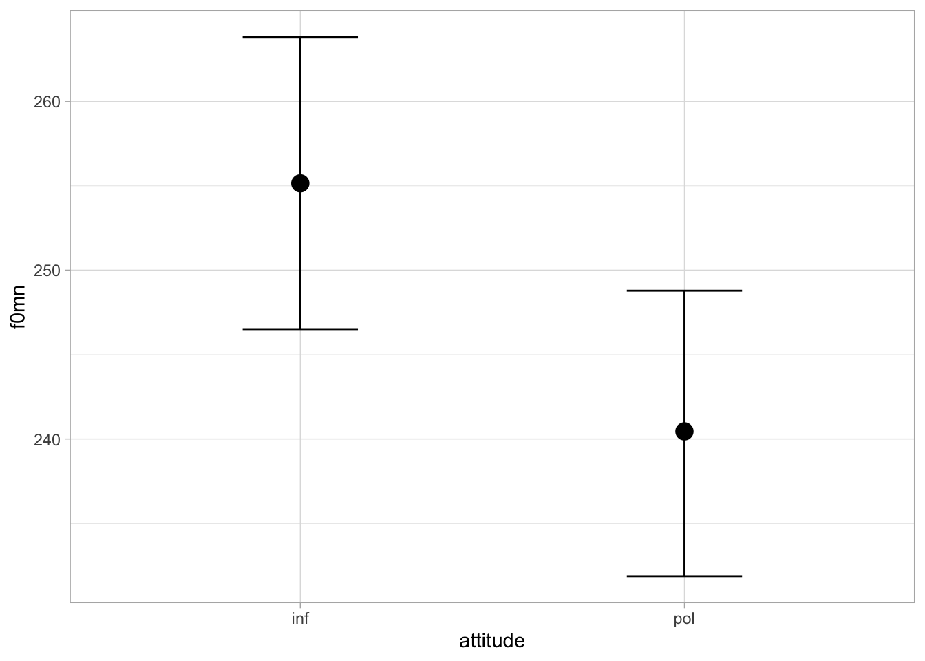
It is worth stressing here that, because of the “averaging across levels” of the “other” predictor, the estimated difference of each predictor is expected to be the same in all levels of the other predictor. We can see this by plotting the expected f0mn based on the model. We use conditional_effects() here for convenience (you will have to plot the posterior distributions from the draws in the exercise below). Figure 34.3 shows the expected predictions of f0mn depending on gender and attitude, separately.
Code
conditional_effects(f0_bm, "gender")
conditional_effects(f0_bm, "attitude")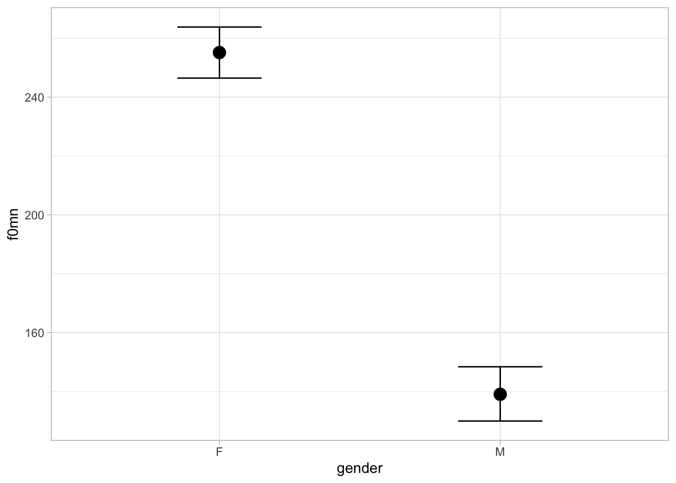
To obtain a single plot that shows the expected f0mn for gender and attitude together, you can specify both predictors separated by a colon gender:attitude. The code below produces Figure 34.4. The order you put the predictors in matters: with gender:attitude, gender is places on the x-axis and attitude is included as a colour aesthetic. Deciding which order to use depends on the data and question: here it makes sense to use gender:attitude since our main question is about attitude.
conditional_effects(f0_bm, "gender:attitude")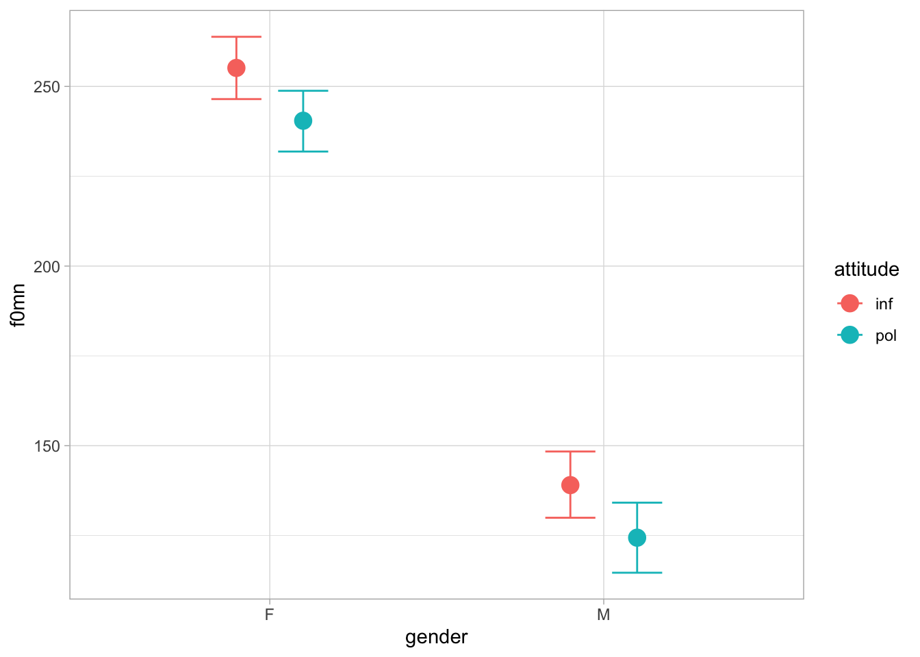
Figure 34.4 should make you appreciate why the effect of attitude is modelled to be the same in female and male participants (and conversely, the effect of gender is the same in informal and polite attitude; you can see this by plotting with the order attitude:gender). If you compare the dots for informal/polite within each gender in the plot, you will notice that the distance between them is basically the same in both genders.
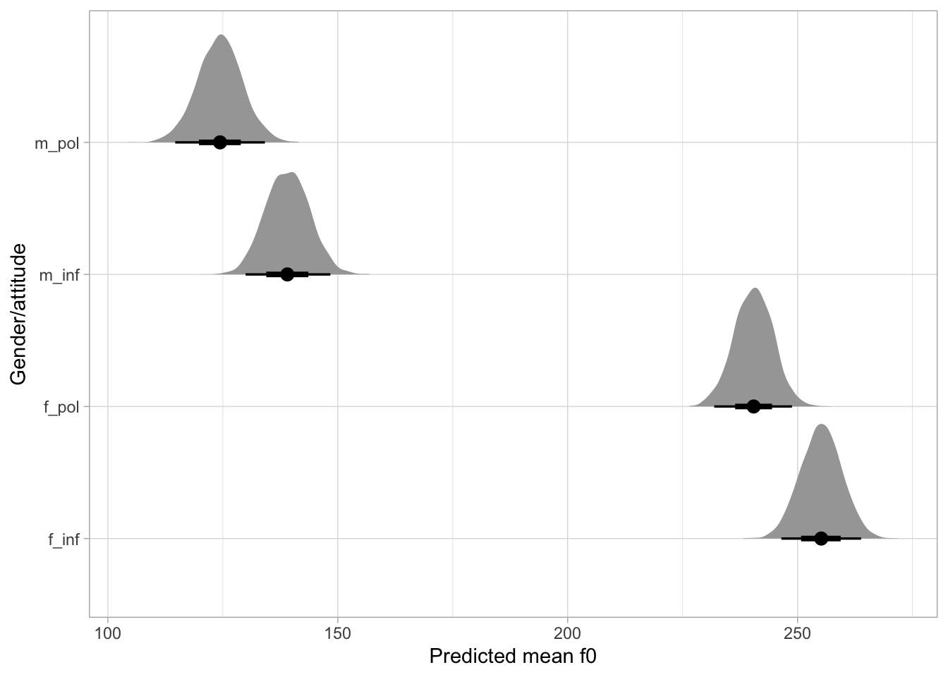
WarningExercise 3
Use as_draws_df() to obtain the model’s draws and recreate the following plot.
The fact that the model is estimating the coefficients for gender and attitude independently from each other begs the question: what if the effect of attitude is not the same in both genders? Based on the data, shown again in Figure 34.5, it seems that the male data does not show much of a difference depending on attitude, as the female data does.
Code
polite_filt |>
  ggplot(aes(gender, f0mn, colour = attitude)) +
  geom_jitter(alpha = 0.7, position = position_jitterdodge(jitter.width = 0.1, seed = 2836))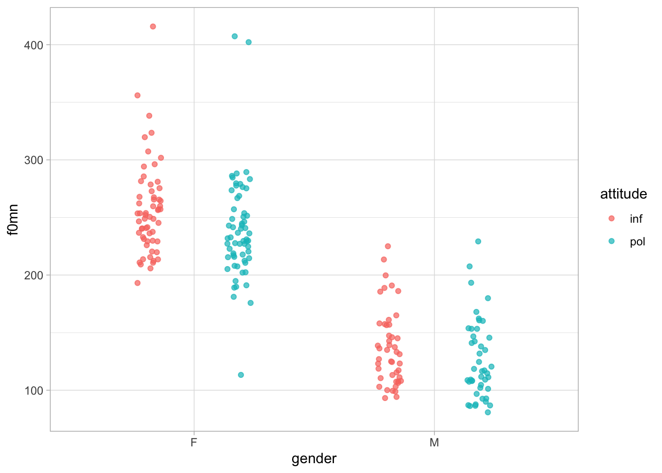
How do we let the model estimate a different effect of attitude based on gender? This is the topic of the next chapter.