glot_status12 Transform data
Data transformation is a fundamental aspect of data analysis. After the data you need to use is imported into R, you will often have to filter rows, create new columns, summarise data or join data frames, among many other transformation operations. In Chapter 11 you have already learned about summarising data, and in this chapter you will learn how to use filter() to filter the data and mutate() to mutate or create new columns.
12.1 Filter rows
Filtering is normally used to filter rows in the data according to specific criteria: in other words, keep certain rows and drop others. Filtering data couldn’t be easier with filter(), from the dplyr package (one of the tidyverse core packages), Let’s work with the coretta2022/glot_status.rds data. Below you can find a preview of the data. Create a new R script called week-03.R and save it in code/. Read the coretta2022/glot_status.rds data.
In the following sections we will filter the rows of the data based on the status column. Before we can move on onto filtering however, we first need to learn about logical operators.
12.1.1 Logical operators
There are four main logical operators, each testing a specific logical statements:
x == y:xequalsy.x != y:xis not equal toy.x > y:xis greater thany.x < y:xis smaller thany.
Logical operators return TRUE or FALSE depending on whether the statement they convey is true or false. Remember, TRUE and FALSE are logical values.
Try the following code in the Console:
# This will return FALSE
1 == 2
[1] FALSE# FALSE
"apples" == "oranges"[1] FALSE# TRUE
10 > 5[1] TRUE# FALSE
10 > 15[1] FALSE# TRUE
3 < 4[1] TRUEYou can use these logical operators with filter() to filter rows that match with TRUE in all the specified statements with logical operators.
12.1.2 The filter() function
Filtering in R with the tidyverse is straightforward. You can use the filter() function. filter() takes one or more statements that return TRUE or FALSE. A common use case is with logical operators. The following code filters the status column so that only the extinct status is included in the new data frame extinct. You’ll notice we are using the pipe |> to transfer the data into the filter() function (you learned about the pipe in Chapter 11). The output of the filter function is assigned <- to extinct. The flow might seem a bit counter-intuitive but you will get used to think like this when writing R code soon enough (although see the R Note box on assignment direction)!
extinct <- glot_status |>
  filter(status == "extinct")

extinct
Neat! extinct contains only those languages whose status is extinct. What if we want to include all statuses except extinct? Easy, we use the non-equal operator !=.
not_extinct <- glot_status |>
  filter(status != "extinct")
not_extinct contains all languages whose status is not extinct. And if we want only non-extinct languages from South America? We can include multiple statements separated by a comma!
south_america <- glot_status |>
  filter(status != "extinct", Macroarea == "South America")
Combining statements like this will give you only those rows where all statements return TRUE. You can add as many statements as you need.
This is all great, but what if we want to include more than one status or macro-area? To do that we need another operator: %in%.
12.1.3 The %in% operator
Try these in the Console:
# TRUE
5 %in% c(1, 2, 5, 7)
[1] TRUE# FALSE
"apples" %in% c("oranges", "bananas")[1] FALSEBut %in% is even more powerful because the value on the left does not have to be a single value, but it can also be a vector! We say %in% is vectorised because it can work with vectors (most functions and operators in R are vectorised).
# TRUE, TRUE
c(1, 5) %in% c(4, 1, 7, 5, 8)
[1] TRUE TRUEstocked <- c("durian", "bananas", "grapes")
needed <- c("durian", "apples")
# TRUE, FALSE
needed %in% stocked[1] TRUE FALSETry to understand what is going on in the code above before moving on.
Now we can filter glot_status to include only the macro-areas of the Global South and only languages that are either “threatened”, “shifting”, “moribund” or “nearly_extinct”.
12.2 Mutate columns
To change existing columns or create new columns, we can use the mutate() function from the dplyr package. To learn how to use mutate(), we will re-create the status column (let’s call it Status this time) from the Code_ID column in glot_status. The Code_ID column contains the status of each language in the form aes-STATUS where STATUS is one of not_endangered, threatened, shifting, moribund, nearly_extinct and extinct. You can check the labels in a column with the unique() function. This function is not from the tidyverse, but it is a base R function, so you need to extract the column from the tibble with $ (the dollar-sign operator). unique() will list all the unique labels in the column (note that it works with numbers too).
unique(glot_status$Code_ID)[1] "aes-shifting" "aes-extinct" "aes-moribund"
[4] "aes-nearly_extinct" "aes-threatened" "aes-not_endangered"We want to create a new column called Status which has only the status part of the label without the aes- part. To remove aes- from the Code_ID column we can use the str_remove() function from the stringr package. Check the documentation of ?str_remove to learn which arguments it uses.
glot_status <- glot_status |>
  mutate(
    Status = str_remove(Code_ID, "aes-")
  )
If you check glot_status now you will find that a new column, Status, has been added. This column is a character column (chr). You see that, as with filter(), you have to assign the output of mutate() to a variable. In the code above we are re-assigning the output to the glot_status variable which we started with. This means that we are overwriting the original glot_status. However, since we have added a new column, we have in practice only added the new column to the old data. If you use the name of an existing column, you will be effectively overwriting that column, so you must be careful with mutate().
Let’s count the number of languages for each endangerment status using the new Status column. You learned about the count() feature in Chapter 11.
glot_status |>
  group_by(Status) |>
  count()
You might have noticed that the order of the levels of Status does not match the order from least to most endangered/extinct. Try count() now with the pre-existing status column (with a lower case “s”). You will get the sensible order from least to most endangered/extinct. Why? This is because status (the pre-existing column) is a factor column with a specified order of the different statuses. A factor column is a column that is based on a factor vector (note that tibble columns are vectors), i.e. a vector that contains a list of values, called levels, from a specified set. Factor vectors (or factors for short) allow the user to specify the order of the values. If the order is not specified, the alphabetical order is used by default. Differently from factor vector/columns, character columns (columns that are character vectors) can only use the default alphabetical order. The Status column we created above is a character column. Check the column type by clicking on the small white triangle in the blue circle next to the name of the tibble in the Environment panel (tip-right panel of RStudio). Next to the Status column name you will see chr, for character. But if you look next to status you will see Factor.
A vector/column can be mutated into a factor column with the as.factor() function. In the following code, we change the existing column Status, in other words we overwrite it (this happens automatically, because the Status column already exists, so it is replaced).
glot_status <- glot_status |>
  mutate(
    Status = as.factor(Status)
  )

levels(glot_status$Status)
[1] "extinct" "moribund" "nearly_extinct" "not_endangered"
[5] "shifting" "threatened" The levels() functions returns the levels of a factor column in the order they are stored in the factor: as mentioned above, by default the order is alphabetical. What if we want the levels of Status to be ordered in a more logical manner: not_endangered, threatened, shifting, moribund, nearly_extinct and extinct? Easy! We can use the factor() function instead of as.factor() and specify the levels and their order in the levels argument.
glot_status <- glot_status |>
  mutate(
    Status = factor(
      Status,
      levels = c("not_endangered", "threatened", "shifting", "moribund", "nearly_extinct", "extinct")
    )
  )

levels(glot_status$Status)
[1] "not_endangered" "threatened" "shifting" "moribund"
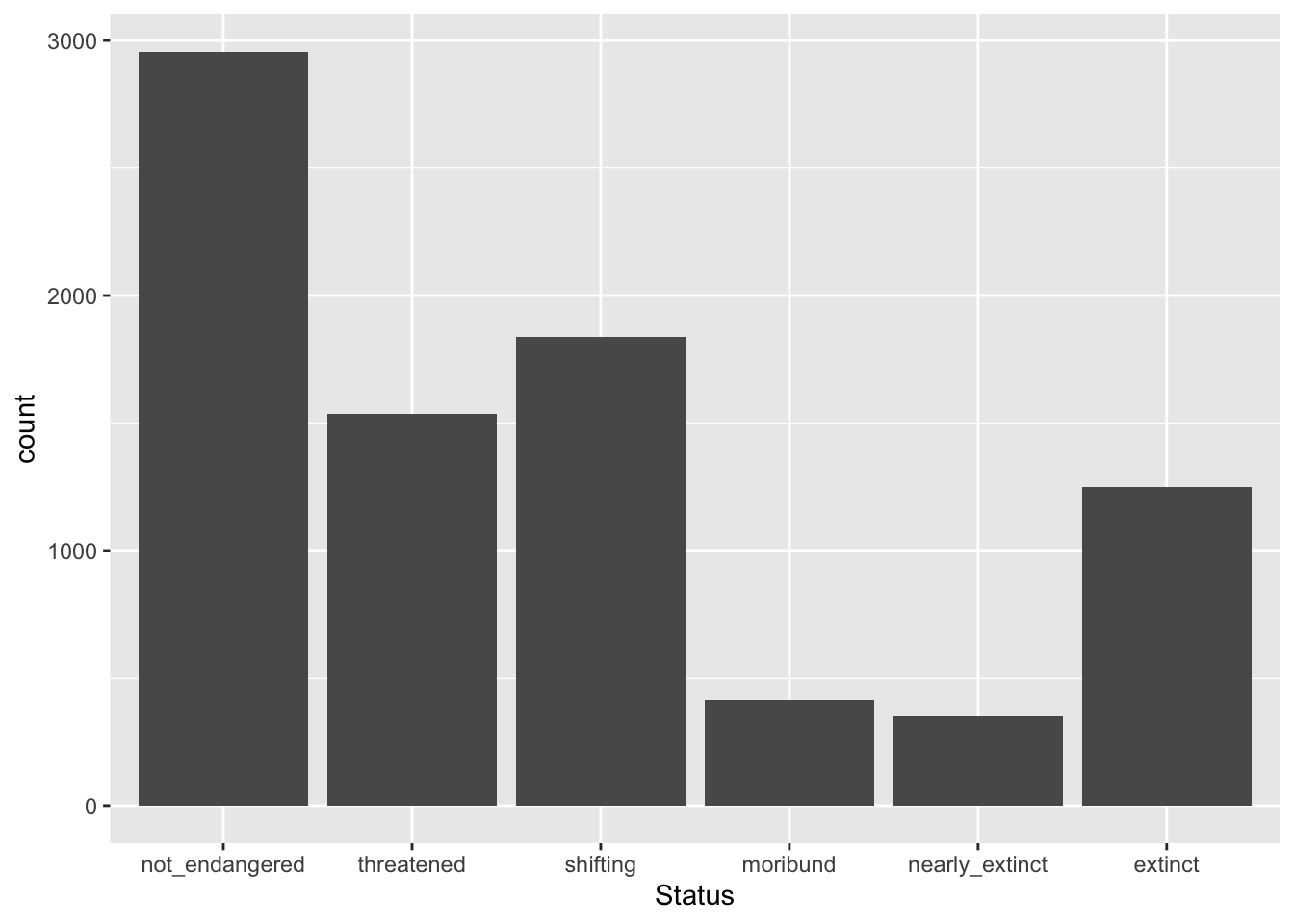
[5] "nearly_extinct" "extinct" You see that now the order of the levels returned by levels() is the one we specified. Transforming character columns to vector columns is helpful to specify a particular order of the levels which can then be used when summarising, counting or plotting.
Here is a preview of data plotting in R, which you will learn in Chapter 15, with the status in the logical order from least to most endangered and extinct.
Code
glot_status |>
  ggplot(aes(x = Status)) +
  geom_bar()