10 Summary measures

10.1 Overview

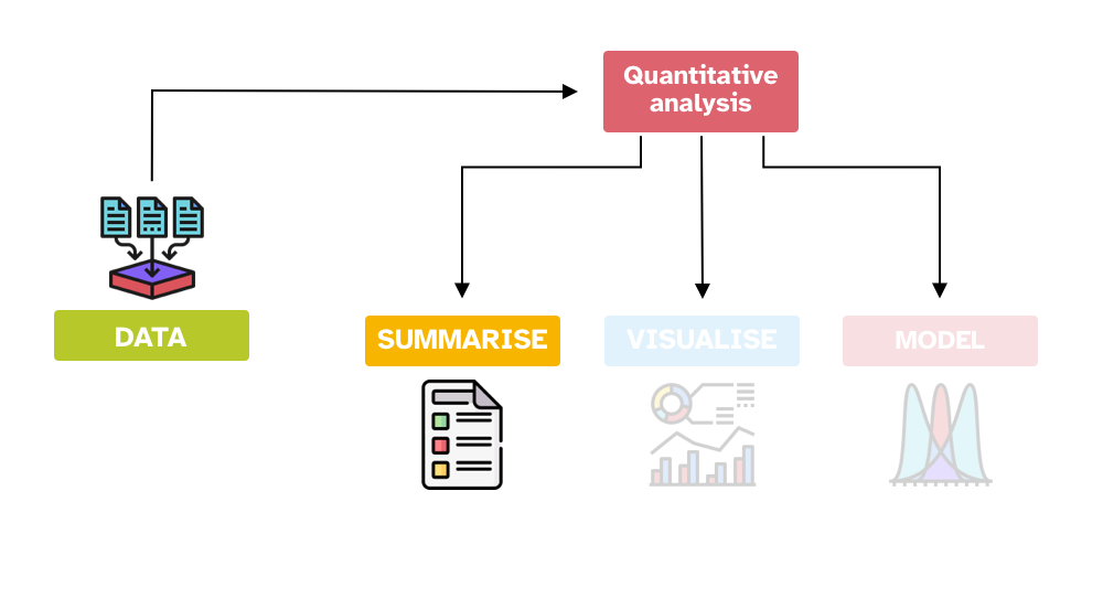
As you learned in Chapter 3, quantitative data analysis can be conceived as three activities: summarising, visualising and modelling data. In this chapter, you will learn about summarising data. When we say “summarising data” we usually mean summarising data variables, by themselves or in group. We can summarise statistical variables using summary measures. There are two types of summary measures.

Measures of central tendency indicate the typical or central value of a variable.
Measures of dispersion indicate the spread or dispersion of the variable values around the central tendency value.

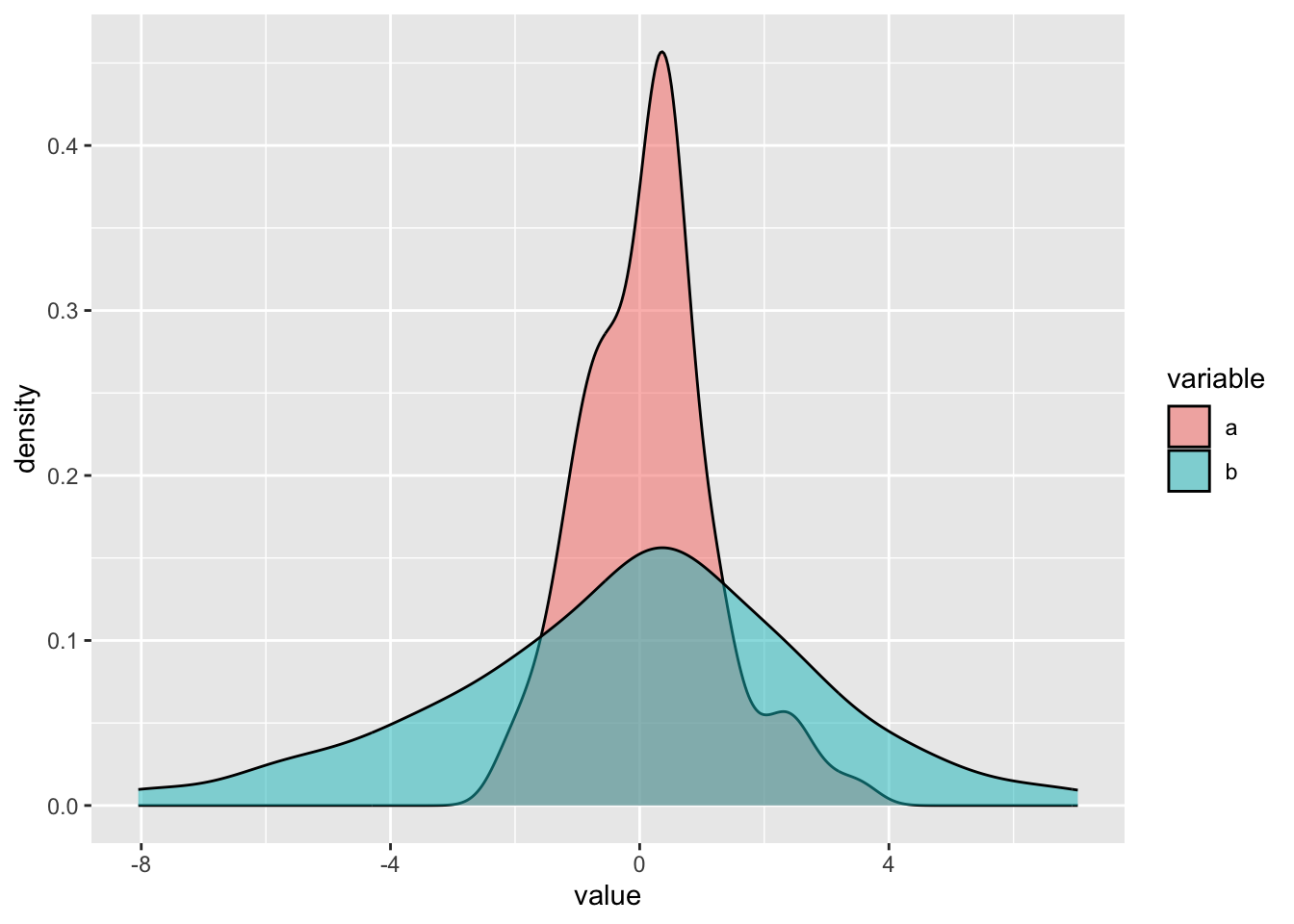
Always report a measure of central tendency together with its measure of dispersion! A central tendency measure captures only one aspect of the “distribution” of the values and variables with the same central tendency value could have very different dispersion, and hence be very different in nature. For example, look at the density plot in Figure 10.1 (you will learn more about them in Chapter 18). These plots are good at showing the distribution of values of numeric variables. The higher the density the curve, the more the values under that part of the curve are represented in the sample. Variable a and b have the same mean (central tendency): the mean is 0. But a has a standard deviation (measure of dispersion, more on this below) of 1 while b’s standard deviation is 3. You can appreciate how different a and b are, despite having exactly the same mean. This should show how important it is to not only report (and think about) central tendencies, like the mean, but also the dispersion of the data around the central tendency.

The following call-outs list common measures of central tendency and dispersions and how they are calculated. You will probably be familiar with most of them and you don’t have to memorise the formulae. The sections after this one will dive into when to use each measure (and how to get them in R), which is much more important.

Measures of central tendency

Mean

\[\bar{x} = \frac{\sum_{i=1}^{n} x_i}{n} = \frac{x_1 + ... + x_n}{n}\]

Median

\[\text{if } n \text{ is odd, } x_\frac{n+1}{2}\]

\[\text{if } n \text{ is even, } \frac{x_\frac{n}{2} + x_{\frac{n}{2}+1}}{2}\]

Mode

The mode is simply the most common value.

Measures of dispersion

Minimum and maximum values

Range

\[ max(x) - min(x)\]

The range is the difference between the largest and smallest value.

Standard deviation

\[\text{SD} = \sqrt{\frac{\sum_{i=1}^n (x_i - \bar{x})^2}{n-1}} = \sqrt{\frac{(x_1 - \bar{x})^2 + ... + (x_n - \bar{x})^2}{n-1}}\]

10.2 Measures of central tendency

A measure of central tendency approximately tells you where the data is most concentrated. There are three common measures of central tendency: mean, median and mode.

10.2.1 Mean

Use the mean with numeric continuous variables, if:

The variable can take on any positive and negative number, including 0.

mean(c(-1.12, 0.95, 0.41, -2.1, 0.09))

[1] -0.354

The variable can take on any positive number only.

mean(c(0.32, 2.58, 1.5, 0.12, 1.09))

[1] 1.122

Important

Don’t take the mean of proportions and percentages!

Better to calculate the proportion/percentage across the entire data, rather than take the mean of individual proportions/percentages: see this blog post. If you really really have to, use the median.

10.2.2 Median

Use the median with numeric (continuous and discrete) variables.

# odd N
median(c(-1.12, 0.95, 0.41, -2.1, 0.09))

[1] 0.09

# even N
even <- c(4, 6, 3, 9, 7, 15)
median(even)

[1] 6.5

# the median is the mean of the two "central" number
sort(even)

[1]  3  4  6  7  9 15

mean(c(6, 7))

[1] 6.5

Important

There are two important characteristics of the mean and the median:

The mean is very sensitive to outliers.
The median is not.

The following list of numbers does not have obvious outliers. The mean and median are not to different.

# no outliers
median(c(4, 6, 3, 9, 7, 15))

[1] 6.5

mean(c(4, 6, 3, 9, 7, 15))

[1] 7.333333

In the following case, there is quite a clear outlier, 40. Look how the mean is higher than the median. This is because the outlier 40 pulls the mean towards it.

# one outlier
median(c(4, 6, 3, 9, 7, 40))

[1] 6.5

mean(c(4, 6, 3, 9, 7, 40))

[1] 11.5

10.2.3 Mode

Use the mode with categorical (discrete) variables. Unfortunately the mode() function in R is not the statistical mode, but rather it returns the R object type.

You can use the table() function to “table” out the number of occurrences of elements in a vector.

table(c("red", "red", "blue", "yellow", "blue", "green", "red", "yellow"))


  blue  green    red yellow 
     2      1      3      2

The mode is the most frequent value: here it is red, with 3 occurrences.

Important

Likert scales are ordinal (categorical) variables, so the mean and median are not appropriate! This is true even when Likert scales are represented with numbers, like “1, 2, 3, 4, 5” for a 5-point scale.

You should use the mode (you can use the median with Likert scales if you really really need to…).

10.3 Measures of dispersion

A measure of dispersion measures how much spread the data is around the measure of central tendency.

10.3.1 Minimum and maximum

You can report minimum and maximum values for any numeric variable.

x_1 <- c(-1.12, 0.95, 0.41, -2.1, 0.09)

min(x_1)

[1] -2.1

max(x_1)

[1] 0.95

range(x_1)

[1] -2.10  0.95

Note that the range() function does not return the statistical range (see next section), but simply prints both the minimum and the maximum.

10.3.2 Range

Use the range with any numeric variable.

x_1 <- c(-1.12, 0.95, 0.41, -2.1, 0.09)
max(x_1) - min(x_1)

[1] 3.05

x_2 <- c(0.32, 2.58, 1.5, 0.12, 1.09)
max(x_2) - min(x_2)

[1] 2.46

x_3 <- c(4, 6, 3, 9, 7, 15)
max(x_3) - min(x_3)

[1] 12

10.3.3 Standard deviation

Use the standard deviation with numeric continuous variables, if:

The variable can take on any positive and negative number, including 0.

sd(c(-1.12, 0.95, 0.41, -2.1, 0.09))

[1] 1.23658

The variable can take on any positive number only.

sd(c(0.32, 2.58, 1.5, 0.12, 1.09))

[1] 0.9895555

Important

Standard deviations are relative and depend on the measurement unit/scale!

Don’t use the standard deviation with proportions and percentages!

10.4 Summary table of summary measures

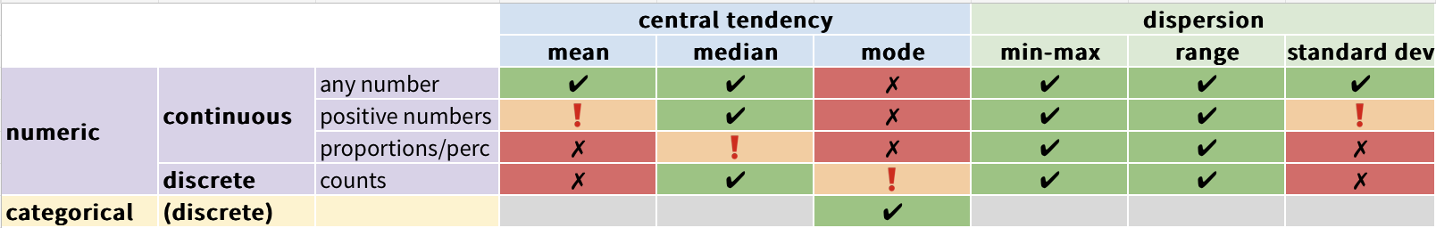
To conclude, here is a table that summarises when each measure should be used, depending on the nature of the variable. You can use this table as a cheat-sheet. Green cells indicate that the measure is appropriate for the variable, red cells indicates that they are not and should not be used, and orange cells indicate you should exercise caution when using those measures with those variables. Gray cells indicate that it’s mathematically impossible to apply that measure to that type of variable.