vow_bm <- brm(
  # `1 +` can be omitted.
  v1_duration ~ speech_rate,
  family = gaussian,
  data = ita_egg_clean,
  cores = 4,
  seed = 20912,
  file = "cache/vow_bm"
)25 Wrangling MCMC draws
![]()
![]()
25.1 MCMC what?
Bayesian regression models fitted with brms/Stan use the Markov Chain Monte Carlo (MCMC) sampling algorithm to estimate the probability distributions of the model’s parameters. You have first encountered MCMC in Chapter 22: the text printed when running brm() is about the MCMC. Bayesian models reconstruct the posterior probability distribution of a set of parameters. More precisely, they reconstruct (i.e. estimate) the joint probability distribution of the parameters. In other words, all parameters are estimated at the same time: think of this as a multidimensional space of probability, with one dimension per parameter. With two parameters, like intercept and slope, this is a 3-dimensional space, something we can imagine: think of a landscape with hills and valleys, where the x-axis are values for the intercept, the y-axis are values for the slope and the z-axis (the vertical axis) are probability densities. The hills represent high probability areas and valleys represent low probability areas. This landscape of hills and valleys is determined by the two components of the Bayes’ Theorem: the prior probability distribution \(P(h)\) and the probability of the data given the prior, \(P(d | h)\).
Constructing the landscape from the prior and data analytically (i.e. solving the mathematical equation of Bayes’ Theorem) is very often very hard or even impossible. The MCMC algorithm allows us to sample points in the landscape without actually mathematically reconstructing the landscape. In the Stan software, which brms uses to fit Bayesian models, the MCMC algorithm uses a specific implementation called Hamiltonian Monte Carlo (HMC). The HMC version of MCMC simulates physical particles rolling through the posterior landscape, using equations from physical mechanics. At each iteration, the algorithm “flicks” a particle (like a pinball ball) and then stops it in its tracks: the place on the posterior landscape where the particle stops is taken as a “draw”. In the 3-dimensional landscape of intercept and slope, the intercept and slope values corresponding to the spot the particle was stopped are recorded. So the draw from one iteration holds one value for the intercept and one for the slope. The algorithm proceeds for several iterations, thus creating a list of draws. These draws can be used to plot and summarise the posterior distributions of the parameters. The draws are called posterior draws, because they come from the posterior probability distribution.
This is a bit abstract and if you want to learn more about MCMC, I recommend McElreath (2020), Ch 9 and Nicenboim, Schad, and Vasishth (2025), Ch 3. Note that to be a proficient user of brms and Bayesian regression models, you don’t need to fully understand the mathematics behind MCMC algorithms, as long as you understand them conceptually.
When you run a model with brms, the draws (i.e. the sampled values) are stored in the model object. All operations on a model, like obtaining the summary(), are actually operations on those draws. We normally fit regression models with four MCMC chains. The sampling algorithm within each chain runs for 2000 iterations by default. The first half (1000 iterations) are used to “warm up” the algorithm (i.e. tune certain parameters related to the mechanics equations that make the particles move) while the second half (1000 iterations) are the ones included in the actual posterior draws. Since four chains run with 2000 iterations of which 1000 are kept as posterior draws, we end up with 4000 draws we can use to learn details about the posterior. The rest of this chapter will teach you how to extract and manipulate the model’s draws. We will do so by revisiting the model fitted in Chapter 24.
25.2 Reproducible model fit
Before we move to the model, it is worth making a couple practical considerations. Fitting simple models with brms is relatively quick. However, more complex model using larger data sets can take some time for the MCMC to efficiently sample the posterior distribution (sometimes even hours!). It is useful to save the model fit to a file so that, once the model is fit once, you don’t have to fit it again. This can be done by specifying a file path in the file argument in the brm() function. I suggest developing the habit of having a dedicated cache/ in your Quarto project to save all of the brms model objects in. Go ahead and create a cache/ folder in your project. Then, in your week-05.qmd document, rewrite the model from the previous chapter like so:
The file argument tells brms to save the model output to the cache/ folder in a file called vow_bm.rds. The extension .rds is appended automatically (this is the same file type you encountered where reading data, like glot_status.rds). What about cores and seed? When the model is fit, four MCMC chains are run. By default, these are run sequentially: the first chain, then the second, then the third and finally the fourth. But we can speed things up a bit by running them in parallel on separate computer cores. Virtually all computers today have at least four cores, so we can run the four chains using four cores. This is what cores = 4 does: it tells brms to run each chain on one core so they are run in parallel. Since the MCMC algorithm contains a random component (physical particles are randomly flicked across the landscape), every time you refit the model, a different set of draws are drawn (because the particles stop at random places in the landscape). One way to make the model reproducible (meaning, obtaining exactly the same draws every time) is to set a “seed”. In computing, a seed is a number used for random number generation: when set, the same list of “random” numbers is produced. The MCMC algorithm uses random number generation to run itself, so by setting the seed we are in fact “fixing” the randomness of the algorithm. The seed number can be any number: here I set it to 20912.
Now run the model. The model will be fitted and the model object will be saved in cache/ with the file name vow_bm.rds. If you now re-run the same code again, you will notice that brm() does not fit the model again, but rather reads it from the file (no output is shown, but trust me, it works!). This saves time: you fit the model once but you can read the output multiple times. This is also good for reproducibility: an independent researcher with access to your code and the cache folder can run your code and get exactly the same results as yours.
25.3 Extract MCMC posterior draws
There are different ways to extract the MCMC posterior draws from a fitted model. In this book, we will use the as_draws_df() function from the posterior package. The function extracts the draws from a Bayesian regression model and outputs them as a data frame. Before we extract the draws from the vow_bm model, let’s revisit the summary.
summary(vow_bm) Family: gaussian
Links: mu = identity; sigma = identity
Formula: v1_duration ~ speech_rate
Data: ita_egg_clean (Number of observations: 3253)
Draws: 4 chains, each with iter = 2000; warmup = 1000; thin = 1;
total post-warmup draws = 4000
Regression Coefficients:
Estimate Est.Error l-95% CI u-95% CI Rhat Bulk_ESS Tail_ESS
Intercept 198.47 3.33 191.76 204.97 1.00 3681 2274
speech_rate -21.73 0.62 -22.93 -20.49 1.00 3623 2421
Further Distributional Parameters:
Estimate Est.Error l-95% CI u-95% CI Rhat Bulk_ESS Tail_ESS
sigma 21.66 0.27 21.14 22.19 1.00 3855 2615
Draws were sampled using sampling(NUTS). For each parameter, Bulk_ESS
and Tail_ESS are effective sample size measures, and Rhat is the potential
scale reduction factor on split chains (at convergence, Rhat = 1).The Draws information in the summary are exactly that: information on the MCMC draws of the model. It says 4 chains were run each with 2000 iterations of which 1000 used for warm-up. thin = 1 just tells brms to keep all the post-warm up draws, and it’s fine as is so you can just ignore it. Then the summary tells us that there are 4000 total post-warm-up draws. We are good to go! We can extract the MCMC draws from the model using the as_draws_df() function. This function returns a data frame (more specifically a tidyverse tibble with class draws_df) with values from each draw of the MCMC algorithm. Since there are 4000 post-warm-up draws, the tibble has 4000 rows.
vow_bm_draws <- as_draws_df(vow_bm)
vow_bm_draws
Ignore the Intercept, lprior and lp__ columns, they are for internal safekeeping. Open the data frame in the RStudio viewer. You will see three extra columns: .chain, .iteration and .draw (which are mentioned in the message printed with the tibble). They indicate:
.chain: The MCMC chain number (1 to 4)..iteration: The iteration number within chain (1 to 1000)..draw: The draw number across all chains (1 to 4000).
Make sure that you understand these columns in light of the MCMC algorithm. The following columns contain the drawn values at each draw for three parameters of the model: b_Intercept, b_speech_rate and sigma. To remind yourself what these mean, let’s have a look at the mathematical formula of the model.
\[ \begin{aligned} vdur & \sim Gaussian(\mu, \sigma) \\ \mu & = \beta_0 + \beta_1 \cdot sr \\ \end{aligned} \]
So:
b_Interceptis \(\beta_0\). This is the mean vowel duration when speech rate is zero.b_speech_rateis \(\beta_1\). This is the change in vowel duration for each unit increase of speech rate.sigmais \(\sigma\). This is the overall standard deviation of vowel duration (the standard deviation of the residual error).
Any inference made on the basis of the model are inferences derived from the draws. One could say that the model “results” are, to put it simply, these draws and that the draws can be used to make inferences about the population one is investigating.
25.4 Summary measures of the posterior draws
The Regression Coefficients table from the summary() of the model reports summary measures calculated from the drawn values of b_Intercept and b_speech_rate. These summary measures are the mean (Estimate), the standard deviation (Est.error) of the draws and the lower and upper limits of the 95% Credible Interval (CrI). We can obtain those same measures ourselves from the data frame with the draws. Let’s calculate the mean and SD of b_Intercept and b_speech_rate (we round to the second digit with round(2)).
# Intercept
mean(vow_bm_draws$b_Intercept) |> round(2)
[1] 198.47sd(vow_bm_draws$b_Intercept) |> round(2)[1] 3.33# Speech rate
mean(vow_bm_draws$b_speech_rate) |> round(2)[1] -21.73sd(vow_bm_draws$b_speech_rate) |> round(2)[1] 0.62Compare the values obtained now with the values in the model summary above. They are the same, because the summary measures in the model summary are simply summary measures of the draws. What if we want to calculate the Credible Intervals (CrIs)? In Chapter 19, you learned about the quantile function (the inverse CDF) to calculate intervals from theoretical distributions. However, here we need to calculate intervals from a sample of posterior draws: the MCMC draws. Note that central probability intervals of posterior draws are called Credible Intervals in Bayesian statistics, so CrI is just a specific type of interval. To obtain intervals from samples we can use the quantile2() function from the posterior package. This function takes two arguments: x, a vector of values to calculate the interval of, and probs, a vector of probabilities, like qnorm(). By default, probs = c(0.05, 0.95). This gives you a 90% CrI interval, but the model summary returns by default a 95% CrI. For a 95% CrI, we need the 2.5th percentile and the 97.5th percentile: c(0.025, 0.975). Here’s the code:
library(posterior)

# Intercept
quantile2(vow_bm_draws$b_Intercept, c(0.025, 0.975)) |> round(2)
q2.5 q97.5
191.76 204.97 # Speech rate
quantile2(vow_bm_draws$b_speech_rate, c(0.025, 0.975)) |> round(2) q2.5 q97.5
-22.93 -20.49 Compare these values with the ones in summary: again they are the same. Remember: a 95% CrI tells us that there is a 95% probability, given the model and data, that the value of the parameters is between the lower and upper limit of the interval. So a 90% CrI tells us that there is an 90% probability that the value is between the lower and upper limit, a 60% interval that there is a 60% probability and so on. We can also say that we are 95% confident that the value lies between the limits. Intervals at lower level of probability are narrower (they span a smaller range of values) than intervals at higher level of probability: so a 95% CrI is always wider than an 80% CrI, which is wider than a 60% CrI and so on. A narrower CrI means more precision: we have a more precise expectation of which range the parameter lies in. But with more precision comes more uncertainty: a 60% CrI is more precise than a 95% CrI because it is narrower, but it is also more uncertain because we go from a 95% probability to a 60% probability. This is the precision/confidence trade-off that we have to live with when doing research. Vasishth and Gelman (2021) say (in the context of frequentist statistics): “[we have to learn] to accept the fact that—in almost all practical data analysis situations—we can only draw uncertain conclusions from data.”
With this model, vow_bm, getting all of these CrIs might look trivial: the 95% CrIs are quite narrow, giving us quite a precise range of values for both the intercept and the coefficient of speech rate. This is because there is quite a lot of data and the model is quite simple, there is only one predictor. With more complex model and smaller data sets, uncertainty is greater and the intervals will span a large range of values. We will see examples later in the book. In those cases, it is helpful to be able to discuss CrIs at different levels of probability, since a lower-probability CrI might tell us something clearer about what we are investigating, while warning us of the increased uncertainty that comes with it.
In the previous chapter, we mentioned that one can calculate the posterior probability of mean vowel duration \(vdur\) based on a specific value of speech rate \(sr\), using the model. We also noted that since we are working with MCMC it is not just like plugging in numbers according to the model’s equation, but rather we need to use the entire probability distributions. In fact, we can use the MCMC draws and plug them in directly, as you would with a single number. However, with MCMC draws the operations in the equation are applied draw-wise. Let’s see what this means by means of code:
vow_bm_draws <- vow_bm_draws |>
  mutate(
    vdur_sr5 = b_Intercept + b_speech_rate * 5
  )
head(vow_bm_draws$vdur_sr5)
[1] 90.46033 89.10209 90.58991 90.38785 90.02444 89.54223The mutate code vdur_sr5 = b_Intercept + b_speech_rate * 5 is based on \(\mu = \beta_0 + \beta_1 sr\). In the code, \(sr\) is set to 5 (syllables per second). So the mean vowel duration when speech rate is 5 syl/s is the intercept \(\beta_0\) plus the slope \(\beta_1\) times 5. Since we are mutating a data frame where each row is one of the 4000 total draws, we are summing and multiplying the values within each row. This gives us a new column vdur_sr5 with 4000 predicted values of vowel duration, one per draw. You can then get summary measures, CrIs and even plot the values of the predicted column, like you would with the coefficients columns. The following code calculates the 95% CrI of the predicted vowel duration when speech rate is 5 syl/s (note we took 5 syl/s just as an example, but you can get prediction for any value of speech rate).
quantile2(vow_bm_draws$vdur_sr5, c(0.025, 0.975)) |> round() q2.5 q97.5
89 91 Based on the model and data, when speech rate is 5 syl/s, the predicted vowel duration is 89-91 ms, at 95% probability.
25.5 Plotting posterior draws
Plotting posterior draws is as straightforward as plotting any data. You already have all of the tools to understand plotting draws with ggplot2. To plot the reconstructed posterior probability distribution of any parameter, we plot the probability density (with geom_density()) of the draws of that parameter. Let’s plot b_speech_rate. This will be the posterior probability density of the change in vowel duration for each increase of one syllable per second. Figure 25.1 shows the posterior probability density of b_speech_rate. If you compare this plot with the central panel of Figure 24.3, the density curves are identical.
vow_bm_draws |>
  ggplot(aes(b_speech_rate)) +
  geom_density() +
  geom_rug(alpha = 0.2)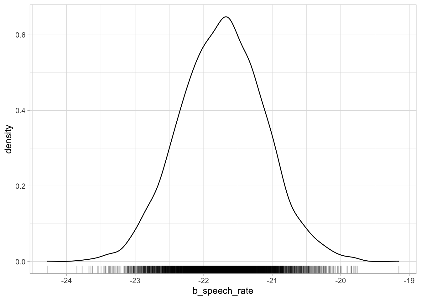
b_speech_rate.
The ggdist package has some convenience ggplot geometries and stats for plotting posterior densities with CrIs. The stat_halfeye() can shade the area under the curve depending on the specified interval levels, like in the code for Figure 25.2 below, which shows 50%, 80% and 95% CrIs. Below the density curve there are error bars of increasing thickness, each corresponding to a CrI. The large dot represents the median of the draws (rather than the mean, like in the model summary). The median is another acceptable summary measure for posteriors.
library(ggdist)

vow_bm_draws |>
  ggplot(aes(x = b_speech_rate)) +
  stat_halfeye(
    .width = c(0.5, 0.8, 0.95),
    aes(fill = after_stat(level))
  ) +
  scale_fill_brewer(na.translate = FALSE) +
  geom_rug(alpha = 0.2)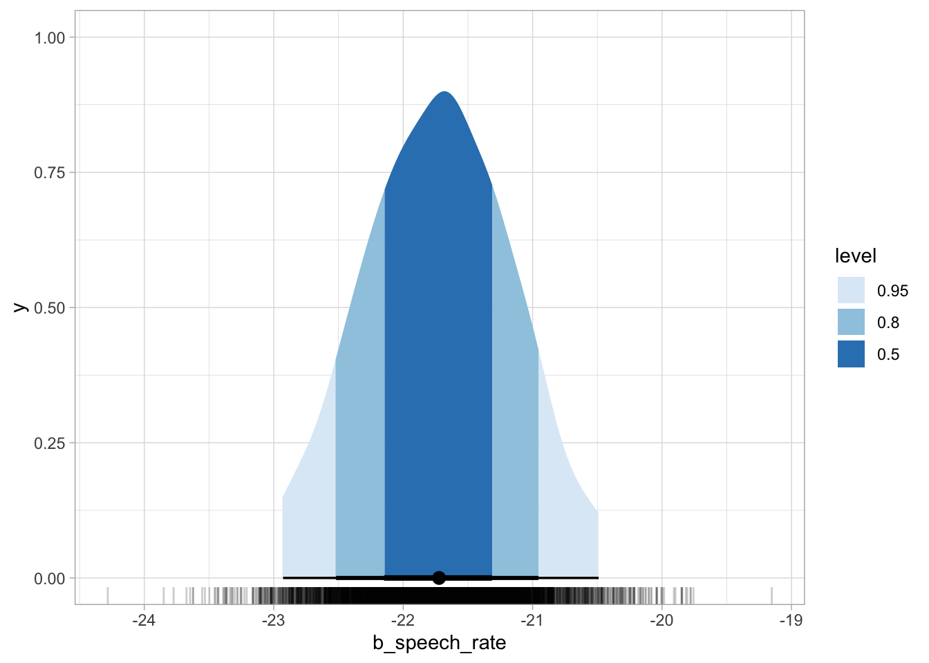
b_speech_rate with credible intervals.
The aes(fill = after_stat(level)) requires a bit of explanation. We are using aes() because we are mapping the fill of the shaded areas to some data, i.e. the level of the CrIs: 0.5, 0.8, 0.95. These are specified in the .width argument. The CrI are calculated by stat_halfeye() from the supplied vow_bm_draws, and the function creates, under the hood, a data frame with the interval limits and a column level which specifies the interval level. So after_stat(level) is simply telling ggplot to use the level column for the fill from the data frame that is available after the stat (the halfeye) has been computed (if you want to know more, you can check the aes_eval documentation from ggplot2). You can learn more about ggdist visualisation tools on the ggdist website.