global_south |>
  ggplot(aes(x = status)) +
...16 More plotting
![]()
16.1 Bar charts
In Figure 12.1 from Chapter 12, you saw how to visualise counts with a bar chart. In this chapter you will learn how to create bar charts with ggplot2. We will first create a plot with counts of the number of languages in global_south (filtered data from coretta2022/glot_status.rds) by their endangerment status and then a plot where we also split the counts by macro-area. To create a bar chart, you use the geom_bar() geometry.
Read the coretta2022/glot_status.rds data and filter it so that you include only languages from Africa, Australia, Papunesia and South America, with any status except not endangered and extinct.
In a simple bar chart, you only need to specify one axis, the x-axis, in the aesthetics aes(). This is because the counts that are placed on the y-axis are calculated by the geom_bar() function under the hood. This quirk is something that confuses many new learners, so make sure you internalise this. Go ahead and complete the following code to create a bar chart.
The counting for the y-axis is done automatically. R looks in the status column and counts how many times each value in the column occurs in the data frame. The counts are then plotted as bars. If you did things correctly, you should get the following plot. The x-axis is now status and the y-axis corresponds to the number of languages by status (count).
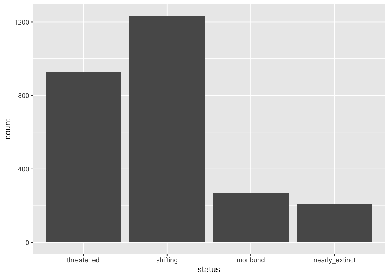
You could write a description of the plot that goes like this:
The number of languages in the Global South by endangered status is shown as a bar chart in Figure 16.1. Among the languages that are endangered, the majority are threatened or shifting.
What if we want to show the number of languages by endangerment status within each of the macro-areas that make up the Global South? Easy! You can make a stacked bar chart.
16.2 Stacked bar charts
A special type of bar charts are the so-called stacked bar charts.
To create a stacked bar chart, you just need to add a new aesthetic mapping to aes(): fill. The fill aesthetic lets you fill bars or areas with different colours depending on the values of a specified column. Let’s make a plot on language endangerment by macro-area. Complete the following code by specifying that fill should be based on status.
global_south |>
  ggplot(aes(x = Macroarea, ...)) +
  geom_bar()
You should get the following.
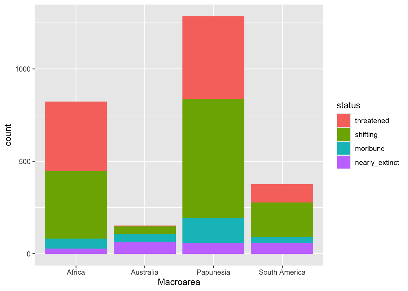
A write-up example:
Figure 16.2 shows the number of languages by geographic macro-area, subdivided by endangerment status. Africa, Eurasia and Papunesia have substantially more languages than the other areas.
16.3 Filled stacked bar charts
In the plot above it is difficult to assess whether different macro-areas have different proportions of endangerment. This is because the overall number of languages per area differs between areas. A solution to this is to plot proportions instead of raw counts. You could calculate the proportions yourself, but there is a quicker way: using the position argument in geom_bar(). You can plot proportions instead of counts by setting position = "fill" inside geom_bar(), like so:
global_south |>
ggplot(aes(x = Macroarea, fill = status)) +
  geom_bar(position = "fill")
The plot now shows proportions of languages by endangerment status for each area separately. Note that the y-axis label is still “count” but should be “proportion”. Use labs() to change the axes labels and the legend name.
global_south |>
ggplot(aes(x = Macroarea, fill = status)) +
  geom_bar(position = "fill") +
  labs(
    ...
)You should get this.
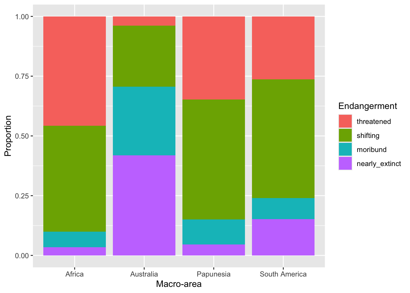
With this plot it is easier to see that different areas have different proportions of endangerment. In writing:
Figure 16.4 shows proportions of languages by endangerment status for each macro-area. Australia, South and North America have a substantially higher proportion of extinct languages than the other areas. These areas also have a higher proportion of near extinct languages. On the other hand, Africa has the greatest proportion of non-endangered languages followed by Papunesia and Eurasia, while North and South America are among the areas with the lower proportion, together with Australia which has the lowest.
16.4 Faceting and panels
Sometimes we might want to separate the data into separate panels within the same plot. We can achieve that easily using faceting. Let’s revisit the plots from Chapter 15. We will use the winter2012/polite.csv data again. This is the plot you previously made. Try and reproduce it by writing the code yourself (you also have to read in the data!).
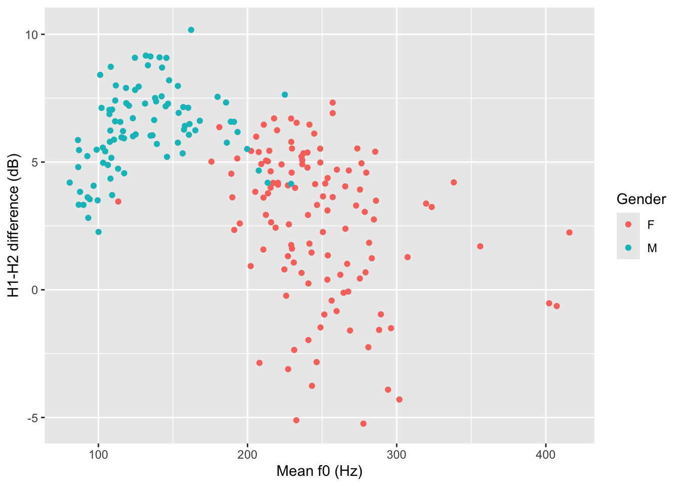
That looks great, but we want to know if being a music student has an effect on the relationship of f0mn and H1H2. In the plot above, the aesthetics mappings are the following: f0mn on the x-axis, H1H2 on the y-axis, gender as colour. How can we separate data further depending on whether the participant is a music student or not (musicstudent)? We can create panels using facet_grid(). This function takes lists of variables to specify panels in rows and/or columns.
Faceting a plot allows to split the plot into multiple panels, arranged in rows and columns, based on one or more variables. To facet a plot, use the facet_grid() function. The syntax is a bit strange. You can specify rows of panels with the rows argument and columns of panels with cols argument, but you have to include column names inside vars(), like this:
polite |>
  ggplot(aes(f0mn, H1H2, colour = gender)) +
  geom_point() +
  facet_grid(cols = vars(musicstudent)) +
  labs(
    x = "Mean f0 (Hz)",
    y = "H1-H2 difference (dB)",
    colour = "Gender"
  )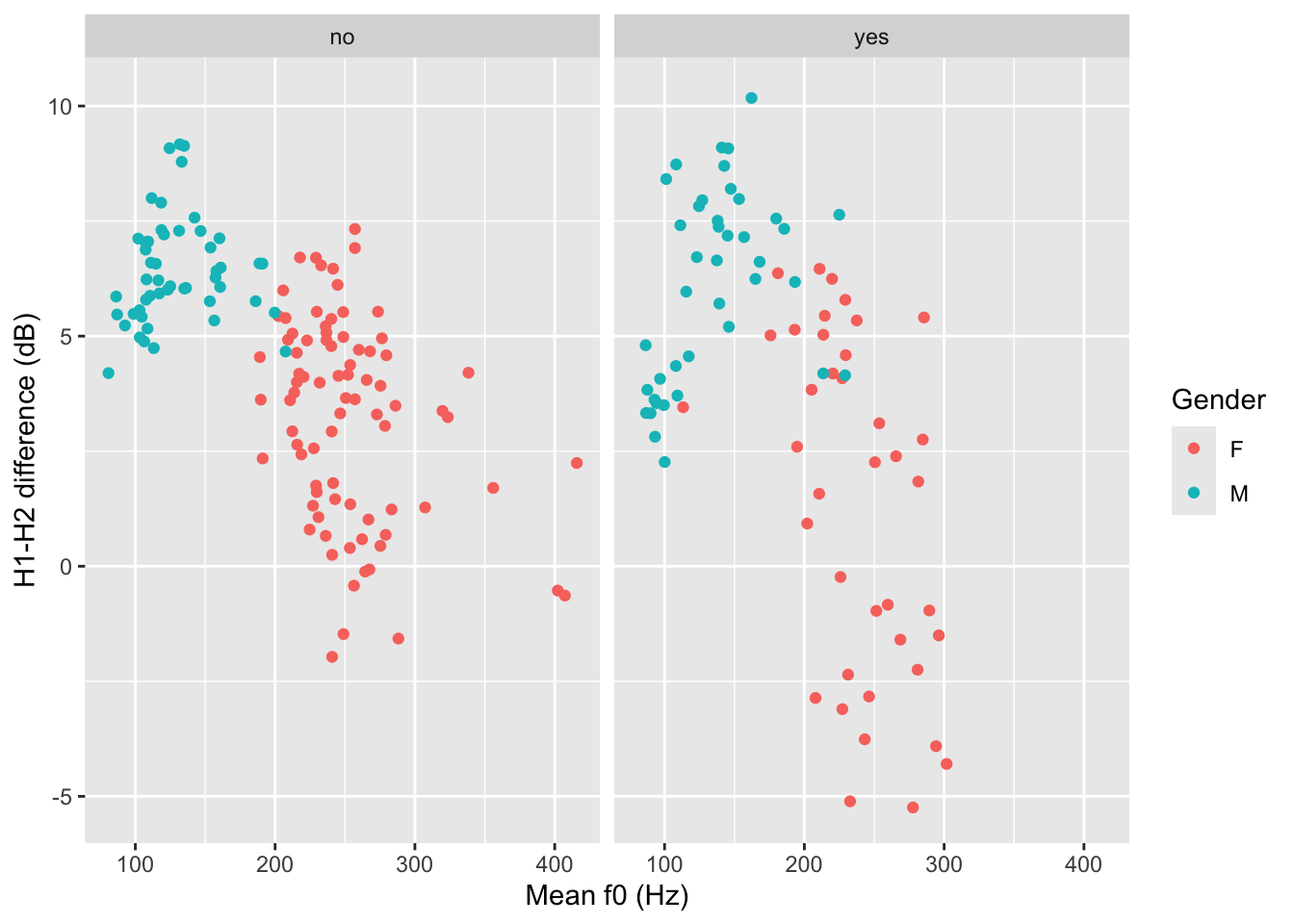
You could write a description of this plot like this:
Figure 16.6 shows mean f0 and H1-H2 difference as a scatter plot. The two panels indicate whether the participant was a student of music. Within each panel, the participant’s gender is represented by colour (red for female and blue for male). Male participants tend to have higher H1-H2 differences and lower mean f0 than females. From the plot it can also be seen that there is greater variability in H1-H2 difference in female music students compared to female non-music participants. Within each group of gender by music student there does not seem to be any specific relation between mean f0 and H1-H2 difference.
The polite data also has a column attitude with values inf for informal and pol for polite. Subjects were asked to speak either as if they were talking to a friend (inf attitude) or to someone with a higher status (pol attitude). Recreate the last plot, this time faceting also by attitude. Use the rows column to create two separate rows for each value of attitude.
polite |>
  ggplot(aes(f0mn, H1H2, colour = gender)) +
  geom_point() +
  facet_grid(cols = vars(musicstudent), rows = ...)