Preface – Quantitative Data Analysis for Linguists in R

Audience

This textbook is specifically designed for the students taking the Quantitative Methods in Linguistics and English Language (QML) course at the University of Edinburgh (UoE), but you don’t have to be enrolled in the course to work through it. This book is an introduction to quantitative methods and statistics in R for absolute beginners in the field of linguistics. No prior familiarity with quantitative methods, statistics or knowledge of R is expected, just a sense of adventure! Of course, the book can be helpful to researchers who have experience with statistics but want to learn about a more modern approach to statistical analysis like Bayesian statistics. Independent of your background, you will be exposed to several aspects of quantitative data analysis and R skills that can be applied and extended to many cases of data analysis in linguistics and related fields.

Justification and pedagogical background

This book is a response to the need for a structured textbook that can fit into a one semester course and yet cover enough materials for an absolute beginner to be able to complete at least basic quantitative analyses. While there are many good books out there, they tend to focus on one aspect or the other, rather than covering all the necessary topics without assuming some prior knowledge. Examples of excellent textbooks are R for Data Science (R4DS, Wickham, Çetinkaya-Rundel, and Grolemund 2023) which covers the basics of R and data processing and visualisation; Statistics for linguists: an introduction using R (Winter 2020), Statistical rethinking: a Bayesian course with examples in R and Stan (McElreath 2020), and Introduction to Bayesian Data Analysis for Cognitive Science (Nicenboim, Schad, and Vasishth 2025), among many others, that focus on statistics with R. In fact, this textbook has taken a lot of inspiration from those books, and I am forever grateful to the authors for their fantastic work.

However, the QML course in the Linguistics and English Language department at UoE is the only quantitative methods course in the department and the majority of students start as absolute beginners. The course must cover basic principles of research methods, some aspects of the philosophy of “science”, statistical concepts, and practical skills in R to run appropriate quantitative analyses. It is a lot to cover and with 9 weeks of teaching available, only the surface can be scratched, but scratched enough that by the end of the course you will feel comfortable taking a further step outside your comfort zone. So this textbook is not in any way meant to be exhaustive and it lives within the constraints of the specifics of the course it is intended to serve. However, where relevant, pointers to other resources will be given so that each reader can choose to focus on some aspects over others.

Another important point about this book is that, like the textbooks mentioned above, it moves away from the “traditional” (perhaps old fashion) way of doing statistics and instead it adopts a fresh take on quantitative data analysis which some have called the “New Statistics” (Cumming 2013; Kruschke and Liddell 2018). All of you view will be familiar with research papers in linguistics (whether you read them for a class or as part of your job as a researcher) and you will surely have encountered the (in)famous p-value and statements like “statistically significant”. These concepts belong to a particular way of doing statistics, called frequentist statistics, which has become ritualised into a set of cookbook recipes that we started to blindly follow (the “Null Ritual,” Gigerenzer 2004, 2018; Gigerenzer, Krauss, and Vitouch 2004). While (good) frequentist statistics is not bad in itself, the so-called Null Ritual has done a lot of damage, as you will learn in later chapters of this book. Because of these and other reasons, this book adopts a Bayesian approach to statistics, where instead of chasing after “significant p-values” we focus on a robust estimation of effects and patterns in the data. This is a bit of an oversimplification, but it should give you enough sense for where the textbook comes from. From a practical perspective, Bayesian statistics just works, even in those cases where the traditional way of doing statistics fails for one reason or the other. By learning a few building blocks of Bayesian statistics, you will be able to extend your skills to develop expertise in more advanced techniques, all within a coherent framework. You will of course learn about p-values and how (not) to interpret them, since a lot of current research is still carried out under the Null Ritualistic approach.

Book structure

The book is structured according to the schedule of the QML course. Chapters are divided into “weeks” and the course will cover those topics weekly. If you are reading this book without being enrolled in the course, you are free to go through the chapters at your own pace! Not however that the chapters are written so that there is a certain progression of topics, and later chapters build on previous ones, so I recommend to start from the first chapter and if need be maybe read through the first chapters quickly if they cover things you are already familiar with, and start reading more intently when you hit a chapter that covers something new.

Each chapter has “badges” that indicate the major topic area of the chapter. While some chapters focus on a specific area, others focus on more than one. These are the badges:

is for chapters on research methods more generally, including research practices and philosophy.
is for chapters that introduce statistical concepts without going necessarily into the details of how to do that in R.
is for chapters that teach you how to use R to complete a particular task, like reading or plotting data, using statistical models or transform data.

The book also uses different types of “call-out boxes” to present specific content. Here are examples.

Definition or hint

A green box contains definitions or hints to solve exercises.

Exercise or activity

Orange boxes are for exercises or more general activities.

Quiz, examples and summaries

Blue boxes contain quizzes, examples or summaries. The title in the box will specify what type of content.

R Note, Spotlight or solutions

Red boxes called “R Note” explain something about R or contain R tips that don’t quite fit in the main text. Spotlight” boxes focus on statistical concepts, historical context or philosophy. Red boxes called “Solutions” are solutions to the exercises.

The textbook will teach how to use R. R is a programming language, meaning that you will have to write code which is executed and the results are returned to (as output in the R Console, as plots, tables, so on). R code in-text will look like this: "this is R code", while longer code chunks will look like this:

# Sum two numbers!

a <- 1 + 2
print(a)

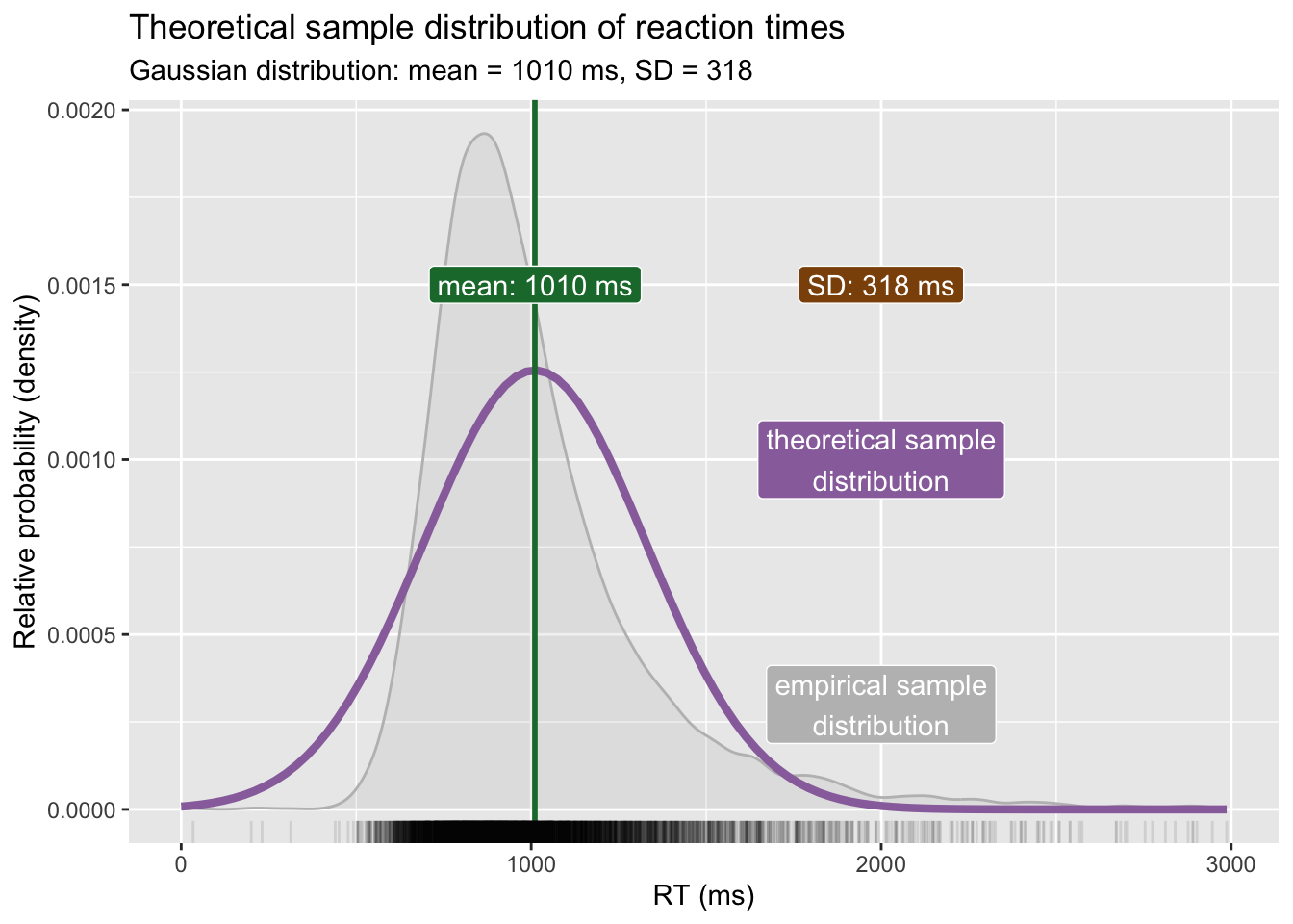
Sometimes, when the R code is not that important, for example for certain plots, you will see a little grey triangle next to Code and if you click on it the code will be shown, like in the following example.

Code

library(tidyverse)
library(glue)
mald <- readRDS("data/tucker2019/mald_1_1.rds")

rt_mean <- mean(mald$RT)
rt_sd <- sd(mald$RT)
rt_mean_text <- glue("mean: {round(rt_mean)} ms")
rt_sd_text <- glue("SD: {round(rt_sd)} ms")
x_int <- 2000

ggplot(data = tibble(x = 0:300), aes(x)) +
  geom_density(data = mald, aes(RT), colour = "grey", fill = "grey", alpha = 0.2) +
  stat_function(fun = dnorm, n = 101, args = list(rt_mean, rt_sd), colour = "#9970ab", linewidth = 1.5) +
  scale_x_continuous(n.breaks = 5) +
  geom_vline(xintercept = rt_mean, colour = "#1b7837", linewidth = 1) +
  geom_rug(data = mald, aes(RT), alpha = 0.1) +
  annotate(
    "label", x = rt_mean + 1, y = 0.0015,
    label = rt_mean_text,
    fill = "#1b7837", colour = "white"
  ) +
  annotate(
    "label", x = x_int, y = 0.0015,
    label = rt_sd_text,
    fill = "#8c510a", colour = "white"
  ) +
  annotate(
    "label", x = x_int, y = 0.001,
    label = "theoretical sample\ndistribution",
    fill = "#9970ab", colour = "white"
  ) +
  annotate(
    "label", x = x_int, y = 0.0003,
    label = "empirical sample\ndistribution",
    fill = "grey", colour = "white"
  ) +
  labs(
    title = "Theoretical sample distribution of reaction times",
    subtitle = glue("Gaussian distribution: mean = {round(rt_mean)} ms, SD = {round(rt_sd)}"),
    x = "RT (ms)", y = "Relative probability (density)"
  )