polite <- read_csv("data/winter2012/polite.csv")

polite_filt <- polite |>
drop_na(f0mn)35 Regression models: interactions
![]()
![]()
The previous chapter explained how to include two predictors in a regression model and how to interpret the results of the model. But we were left wondering: what if the effect of attitude differs between the two genders? In this chapter we will talk about interactions: regression models can estimated different effects of one predictor depending on the levels of the other other predictor, by adding a so-called interaction term. Keep reading to learn about them.
35.1 Is the effect of attitude modulated by gender?
Let’s start by reading and filtering the polite data (Winter and Grawunder 2012). We drop NA values from the f0mn column.
Figure 35.1 shows once again the mean f0 values split by gender and attitude. In principle, we have no reason to expect that the effect of attitude will be the same in both genders, and conversely we have no reason to expect the opposite (that it will be different). The best way forward in regression modelling is to allow the model to estimate the (possible) difference: depending on the results, you will be able to report the estimated difference and reason as to whether the difference is meaningful or not.
Code
polite_filt |>
  ggplot(aes(gender, f0mn, colour = attitude)) +
  geom_jitter(alpha = 0.7, position = position_jitterdodge(jitter.width = 0.1, seed = 2836))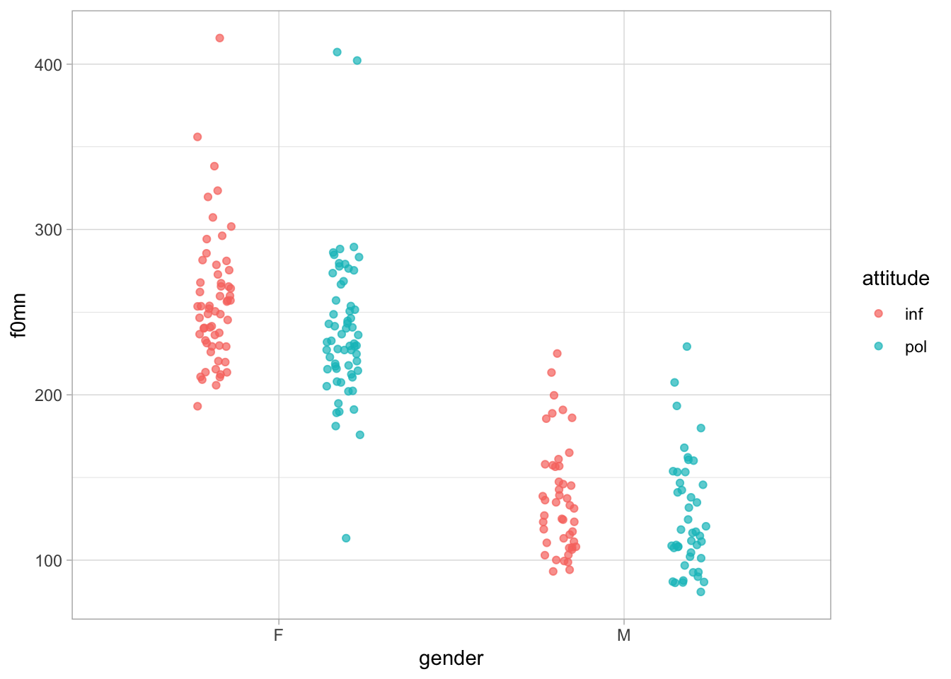
35.2 Interaction terms
To allow a regression model to estimate “interactions” between predictors, or in other words to estimate different effects of one predictors based on the levels of the other, we need to include so-called interaction terms. An interaction term, is a model term that tells the model to estimate interactions. Before we see how to include interaction terms in R/brms, let’s go through the model’s formula.
We will model mean f0 f0mn as a function of gender and attitude and an interaction between the two. Here is what the formula looks like:
\[ \begin{aligned} f0mn_i & \sim Gaussian(\mu_i, \sigma)\\ \mu_i & = \quad \beta_0 \\ & \quad + \beta_1 \cdot gen_{\text{M}[i]} \\ & \quad + \beta_2 \cdot att_{\text{POL}[i]} \\ & \quad + \beta_3 \cdot gen_{\text{M}[i]} \cdot att_{\text{POL}[i]} \end{aligned} \]
There are now not just three \(\beta\) coefficients, but four: \(\beta_0, \beta_1, \beta_2, \beta_3\). The new coefficient that we haven’t seen before is \(\beta_3\). This is the coefficient of the interaction term of gender and attitude. Let’s work out the formula of \(\mu\) depending on the combinations gender and attitude: remember that \(gen_\text{M}\) is 0 for female and 1 for male, and \(att_\text{POL}\) is 0 for informal and 1 for polite.
| female and informal | \(\beta_0\) |
| male and informal | \(\beta_0 + \beta_1\) |
| female and polite | \(\beta_0 + \beta_2\) |
| male and polite | \(\beta_0 + \beta_1 + \beta_2 + \beta_3\) |
We get this because when either \(gen_\text{M}\) or \(att_\text{POL}\) are 0, the corresponding \(\beta\) coefficient gets dropped from the equation. Importantly, notice how for male/polite we need all four coefficients. For male and polite mean f0, we need the coefficient for male \(\beta_1\) and that for polite \(\beta_2\), but also the interaction coefficient \(\beta_3\) because in this combination \(gen_\text{M}\) and \(att_\text{POL}\) are both 1. You can thing of \(\beta_3\) as the “adjustment” to the individual effects of gender = male and attitude = polite. In other words, the interaction coefficient \(\beta_3\) tells you how the combined effects of gender = male and attitude = polite differ from their simple sum (i.e. \(\beta_1 + \beta_2\)).
Moving on to R, we can include an interaction term between gender and attitude in the R formula with gender:attitude (the two predictors separated by a colon :).
f0_bm_int <- brm(
  f0mn ~ gender + attitude + gender:attitude,
  family = gaussian,
  data = polite,
  cores = 4,
  seed = 7123,
  file = "cache/ch-regression-interaction_f0_bm_int"
)
Note that there is a syntactic sugar for interactions: instead of writing in full gender + attitude + gender:attitude you can just write gender * attitude (the two predictors separated by a star *). The “star” syntax expands to the full syntax. It is up to you which syntax you use, although for beginners I suggest using the longer one for clarity. Run the model now.
Getting a regression model to estimate interactions is easy, but a warning: because we have included an interaction in the model, the interpretation of the coefficients has changed slightly relative to how we interpret the coefficients of categorical predictors in models without interactions!
35.3 Interpreting models with interactions
Let’s look at the model summary. With interactions, the coefficients of categorical predictors are interpreted slightly differently than when there are no interactions.
summary(f0_bm_int) Family: gaussian
Links: mu = identity; sigma = identity
Formula: f0mn ~ gender + attitude + gender:attitude
Data: polite (Number of observations: 212)
Draws: 4 chains, each with iter = 2000; warmup = 1000; thin = 1;
total post-warmup draws = 4000
Regression Coefficients:
Estimate Est.Error l-95% CI u-95% CI Rhat Bulk_ESS Tail_ESS
Intercept 256.56 5.20 246.38 267.27 1.00 2632 2950
genderM -119.38 7.66 -134.08 -104.50 1.00 2532 2665
attitudepol -17.48 7.28 -31.76 -3.18 1.00 2573 2806
genderM:attitudepol 6.65 10.67 -14.20 27.47 1.00 2191 2693
Further Distributional Parameters:
Estimate Est.Error l-95% CI u-95% CI Rhat Bulk_ESS Tail_ESS
sigma 39.10 1.94 35.52 43.14 1.00 3834 2779
Draws were sampled using sampling(NUTS). For each parameter, Bulk_ESS
and Tail_ESS are effective sample size measures, and Rhat is the potential
scale reduction factor on split chains (at convergence, Rhat = 1).Interceptis \(\beta_0\): this is, as you would expect, the mean f0 when gender and attitude are at their reference levels, i.e. female and informal. According to the model, there is a 95% probability that the mean f0 is between 246 and 267 Hz with female speakers and informal attitude.genderMis \(\beta_1\): this is the difference in mean f0 between male and female gender, when attitude is informal (i.e. at the reference level of attitude). This differs from the interpretation in models with no interactions where instead the coefficient would capture the average difference between male and female gender. According to the model, the mean f0 is 105 to 134 Hz lower in male than in female participants, when the attitude is informal.attitudepolis \(\beta_2\): this is the difference in mean f0 between polite and informal attitude, when gender is female (i.e. at the reference level of gender). This also differs from the interpretation in models with no interactions where instead the coefficient would capture the average difference between polite and informal attitude. According to the model, the mean f0 is 3 to 32 Hz lower in polite than in informal speech, in female speakers.genderM:attitudepolis \(\beta_3\): this is the interaction coefficient. This coefficient tells you the adjustment you have to make to the effects of gender and attitude (so \(\beta_1 +\beta_2 + \beta_3\)), on top of what is predicted by the additive effects of gender and attitude (so \(\beta_1 + \beta_2\)). According to the model, the difference between female informal and male polite speech differs from the additive effect of gender and attitude by -14 to +27 Hz, at 95% confidence. The 95% CrI [-14, +27] spans both negative and positive values: there is uncertainty as to whether the effect of attitude differs in the two genders (and, symmetrically, whether the effect of gender differs in informal and polite speech), and as to weather the difference is positive or negative. The interval might indicate that a positive difference is more likely, given that the interval spans a wider range of positive values than negative values.
Let’s extract the model’s draws and process them to get summary measures and relevant plots.
35.4 Model’s draws and expected predictions
We can extract the draws from the model object as usual.
f0_bm_int_draws <- as_draws_df(f0_bm_int)To calculate the expected predictions of f0, we plug in the columns from the draws object f0_bm_int_draws according to the model’s formula. To name the new columns with the expected predictions, we use f for female and m for male for gender, and inf for informal and pol for polite for attitude. Note that, since the name of interaction coefficient b_genderM:attitudepol contains a colon :, we need to surround it with back-ticks to prevent R for interpreting the colon : as the range operator (like in 1:5, which returns integers from 1 to 5).
f0_bm_int_draws <- f0_bm_int_draws |>
  mutate(
    # \beta_0
    f_inf = b_Intercept,
    # \beta_0 + \beta_1
    f_pol = b_Intercept + b_attitudepol,
    # \beta_0 + \beta_2
    m_inf = b_Intercept + b_genderM,
    # \beta_0 + \beta_1 + \beta_2 + \beta_3
    m_pol = b_Intercept + b_genderM + b_attitudepol + `b_genderM:attitudepol`
  )
Let’s plot the distributions of the expected predictions we just calculated. We need to pivot the draws object: to make plotting easier, we need a column with the gender value and one column with the attitude value, and also a column with the expected prediction values. We can split the cond column with separate() from dplyr. This function splits strings by punctuation characters, like _, so it works with strings like f_inf, which gets split into f and inf. The two new values are input into the specified new columns gender and attitude (the user picks and specifies the names as one of the arguments).
f0_bm_int_epred <- f0_bm_int_draws |>
  # First, select only the columns we need to pivot
  select(f_inf:m_pol) |>
  # From wide to long
  pivot_longer(f_inf:m_pol, names_to = "cond", values_to = "epred") |>
  # Split `cond` column to make a gender and an attitude column
  separate(cond, c("gender", "attitude"))

f0_bm_int_epred
Now we can plot the expected predictions with ggplot2 (Figure 35.2). We set scales = "free_x" in facet_grid() to allow ggplot to use different scales in the x-axis (try to run the code without specifying the scales argument to see why).
f0_bm_int_epred |>
  ggplot(aes(epred, attitude)) +
  stat_halfeye() +
  facet_grid(cols = vars(gender), scales = "free_x")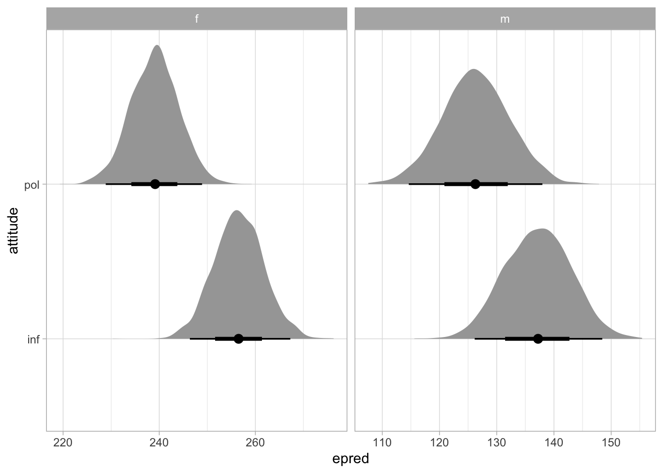
An alternative to stat_halfeye() is stat_interval(). By default, it plots the 50-80-95% CrIs of the expected predictions.
f0_bm_int_epred |>
  ggplot(aes(attitude, epred)) +
  stat_interval() +
  facet_grid(cols = vars(gender))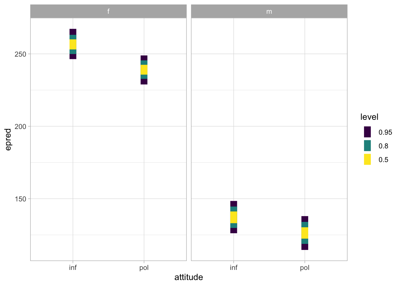
We can observe two main things:
The f0 of female participants is generally higher than that of male participants.
In both genders, f0 is somewhat higher in informal than in polite speech.
Possibly, the attitude difference is somewhat larger in female than in male participants.
These general observations can be quantified using CrIs from the model. For example, the 95% CrI of the \(\beta_3\) coefficient suggests a good amount of uncertainty in how the attitude effect differs between female and male participants. Furthermore, we can compute summary measures of the attitude difference in male participants directly.
f0_bm_int_draws |>
  mutate(
    m_pol_inf = m_pol - m_inf
  ) |>
  summarise(
    mean_diff = mean(m_pol_inf), sd_diff = sd(m_pol_inf),
    lo_diff = quantile2(m_pol_inf, probs = 0.025),
    hi_diff = quantile2(m_pol_inf, probs = 0.975)
  ) |>
  round()
The mean difference is -11 Hz (SD = 8) and the 95% CrI is [-27, +5] Hz. This is somewhat indicative of a difference (polite speech is produced with a somewhat lower f0) but it is also possible that there is instead a negligible positive difference (+5 Hz). Comparing this with the effect of attitude in female participants (as given by \(\beta_2\) or attitudepol) which is at 95% confidence between -32 to -3 Hz, we cannot really argue for or against the effect of attitude being different in the two genders. In other words, we are left with a certain level of uncertainty.