3 Methods
Each of the proposals regarding the origin of the voicing effect, reviewed in 1, stresses one particular aspect of the mechanisms that could lie behind this phenomenon. Whereas some of the hypotheses concern biases of the perceptual system, others depend on articulatory and aerodynamic properties of speech production. Crucially, all accounts have found only partial support in the literature. Over the years, evidence has accumulated for the articulatory accounts based on compensatory temporal adjustments, laryngeal adjustments, and rate of consonant closure. Given the complex nature that characterises the production accounts, this thesis sets out to investigate durational and dynamic aspects of the articulation of vowel-consonant sequences. The outcomes of a time-synchronised analysis of acoustic and articulatory data from Italian and Polish (3.1) indicate that components of temporal compensation and gestural phasing are the likely source of the differences in vowel and closure durations. A follow-up acoustic study of English (3.2) further corroborates these results, and offers new insights on the possible development of the voicing effect from the word-level structuring of vocalic and consonantal gestures.
An overview of these studies, with information on experimental materials, procedures, and data processing, is given in this chapter. The following sections constitute a synopsis of the methodologies presented in more specific details in the relevant papers. The data and code referred to here can be found in the dissertation repositories on the Open Science Framework and GitHub (see 3.3.4). Ethics clearance to undertake this work was obtained from the University Research Ethics Committee (UREC) of the University of Manchester (REF 2016-009976).
3.1 Exploratory study of the voicing effect in Italian and Polish (Study I)
As discussed in 2.1, since the accounts this dissertation focusses on cover aspects of segmental duration, consonantal articulatory gestures, and voicing, data was obtained from three sources: (1) acoustics, (2) ultrasound tongue imaging, a non-invasive technique to image the tongue using ultrasonic equipment, and (3) electroglottography, an indirect and safe method to gather information on vocal fold activity. In the following sections, I offer an outline of the methodologies employed in Study I, while referring the reader to specific papers for a more in-depth description.
3.1.1 Participants
A total of 17 participants were recruited in Manchester (UK) and in Verbania (Italy). Eleven were native speakers of Italian (IT01-IT05, IT07, IT09, IT11-IT14), and six of Polish (PL02-PL07). Missing speaker codes refer to test participants or participants that produced unusable data because of individual anatomy or recording issues. Recordings were made in a sound-attenuated room at the Phonetics Laboratory of the University of Manchester, or in a quiet room at a field location in Verbania (IT03-IT07). Due to technical issues or poor signal quality, ultrasonic data of /u/ from two speakers (IT07, PL05) and electroglottographic data from two others (IT04, IT05) are missing. Participants’ sociolinguistic data is given in 4. The participants were given an information sheet prior to the experiment and signed a consent form.
3.1.2 Ultrasound tongue imaging and electroglottography
2D Ultrasound tongue imaging (UTI) uses ultrasonography for charting the movements of the tongue into a two-dimensional image (Gick 2002; Stone 2005; Lulich, Berkson & Jong 2018). In medical sonography, ultrasonic waves (sound waves at high frequencies, ranging between 2 and 14 MHz) are emitted from piezoelectric components in a transducer. The surface of the transducer is placed in contact with the subject’s skin, and the waves irradiate from the transducer in a fan-like manner, travelling through the subject’s soft tissue. When the surface of a material with different density is hit by the ultrasonic waves, some of the waves are partially reflected, and such ‘echo’ is registered by the probe. The information interpolated from these echoes can be plotted on a two-dimensional graph, where different material densities are represented by different shades (higher densities are brighter, while lower densities are darker). The graph, or ultrasound image, shows high density surfaces as very bright lines, surrounded by darker areas. By positioning the ultrasound probe in contact with the sub-mental triangle (the surface below the chin), sagittally oriented, it is possible to infer the cross-sectional profile of the tongue, which appears as a bright line in the resulting ultrasound image.
Electroglottography (Fabre 1957; Childers & Krishnamurthy 1985; Scherer & Titze 1987; Rothenberg & Mahshie 1988) is a technique that measures the size of contact between the vocal folds (the Vocal Folds Contact Area, VFCA). A high frequency low voltage electrical current is sent through two electrodes which are in contact with the surface of the neck, one on each side of the thyroid cartilage. The impedance of the current is directly correlated with VFCA, while its amplitude is inversely correlated with it (Titze 1990). Impedance increases with lower VFCA and decreases with higher VFCA. Conversely, amplitude decreases when the VFCA increases and it increases when the VFCA decreases. The EGG unit registers changes in impedance and converts it into amplitude values. The unit outputs a synchronised stereo recording which contains the EGG signal from the electrodes in one channel and the audio signal from the microphone in the other.
3.1.3 Equipment set-up
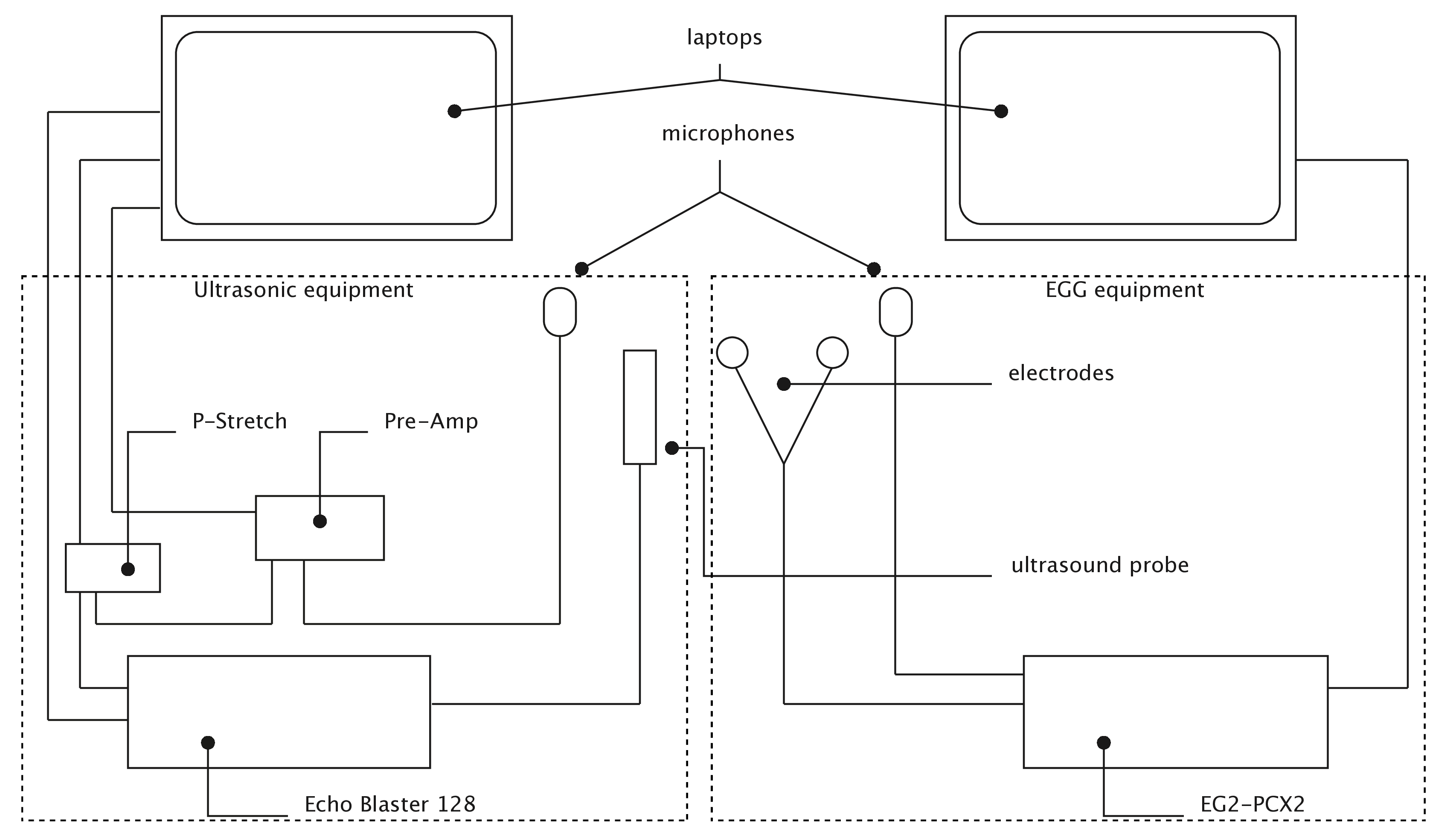
Figure 3.1: Schematics of the equipment set-up of Study I. Stabilisation headset not shown.
Figure 3.1 shows a schematics of the equipment set-up used in this study. The left part of the figure shows the ultrasonic components (Articulate Instruments Ltd 2011), while the EGG components (Glottal Enterprises) are shown on the right. Two separate Hewlett-Packard ProBook 6750b laptops with Microsoft Windows 7 were used for the acquisition of the UTI and EGG recordings. The main ultrasonic component was a TELEMED Echo Blaster 128 unit with a TELEMED C3.5/20/128Z-3 ultrasonic transducer (20mm radius, 2-4 MHz), plugged into one laptop via a USB cable. A P-Stretch unit (used for signal synchronisation) was connected to the ultrasound unit via a custom modification (Articulate Instruments Ltd 2011). The P-Stretch unit and a Movo LV4-O2 Lavalier microphone fed into a FocusRight Scarlett Solo pre-amplifier, which was plugged into the ultrasound laptop via USB. A second Movo microphone and the electrodes were connected to a Glottal Enterprises EG2-PCX2 unit, which was plugged into the second laptop (the audio signals from the UTI and the EGG units were used for synchronisation, see below).
The subject wore a metallic headset produced by Articulate Instruments Ltd (2008) (Figure 3.2), which stabilises the position of the ultrasound probe (allowing free head movement), and the Velcro strap with the EGG electrodes around their neck. The electrodes were located on each side of the thyroid cartilage, at the level of the glottis. The microphones were clipped to the headset on either side, at identical heights. Before the reading task, the participant’s occlusal plane was obtained using a bite plate (Scobbie et al. 2011). This procedure allows data to be rotated along the occlusal plane and provides us with a reference plane.
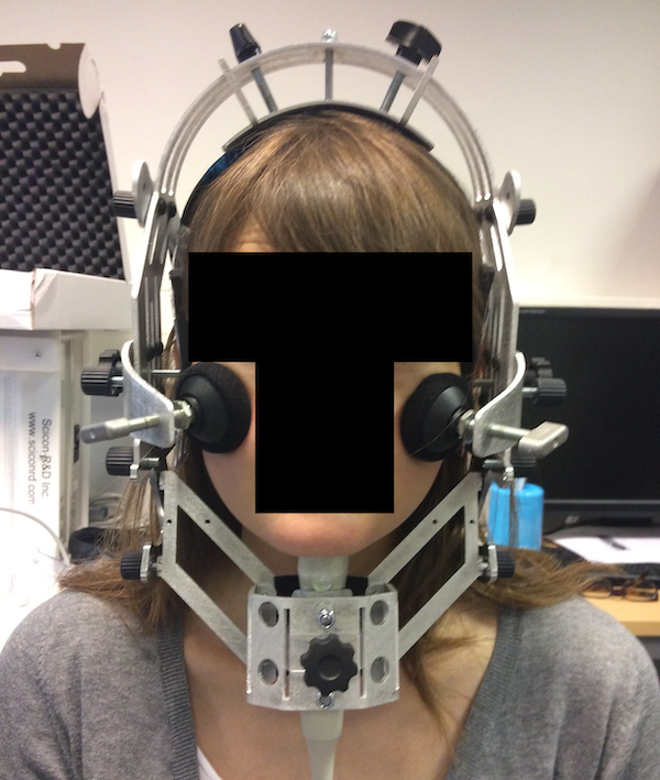
Figure 3.2: Ultrasonic probe stabilisation headset.
3.1.4 Procedure and data processing
The participants read sentence stimuli containing test words presented on the screen via the software Articulate Assistant Advanced™ (AAA v2.17.2, Articulate Instruments Ltd (2011))). The test words were CVCV words, where C = /p/, V = /a, o, u/, C = /t, d, k, g/, and V = V. Note that in both languages C2 is the onset of the second syllable. The choice of the segmental make-up of the test words was constrained by the use of ultrasound tongue imaging. The words were embedded in the frame sentence Dico X lentamente ‘I say X slowly,’ and Mówię X teraz ‘Say X now’ for Italian and Polish respectively. 4 provides more details on the rationale behind the material design.
The UTI+audio and EGG+audio signals were acquired and recorded by means of AAA and Praat (Boersma & Weenink 2018) respectively.
Since the signals from the ultrasonic machine and the electroglottograph are recorded simultaneously but separately, data from both sources were synchronised after acquisition.
Synchronisation was achieved using the cross-correlation of the audio signals obtained from the separate sources (Grimaldi et al. 2008).
The interval between the start of the cross-correlated signal and the time of the signal maximum amplitude is equal to the lag between the two original sounds (Figure 3.3).
Synchronisation of the original sound files was achieved by trimming the beginning of the longer sound by the lag obtained from cross-correlation.
A Praat script was written to automate the synchronisation process (sync-egg.praat in Coretta 2018a).
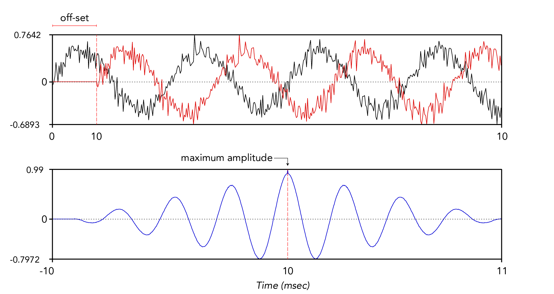
Figure 3.3: Synchronisation of two sounds by cross-correlation. The top panel shows the waveforms of two identical sounds, one of which has been offset by 10 ms. The bottom panel shows the cross-correlation of the two sounds in the top panel. The offset of the sounds corresponds to the time of maximum amplitude in the cross-correlated sound.
A time-aligned transcript of the recordings was obtained with a force-alignment procedure using the SPeech Phonetisation Alignment and Syllabification (SPPAS) software (Bigi 2015). SPPAS is a language-agnostic system which comes with pre-packaged models for a variety of languages, among which Italian, Polish, and English. Since the audio recorded with the EGG system was nosier than that recorded with the UTI system, the latter was used in all subsequent acoustic-based analyses. The output of the force-alignment is a Praat TextGrid with time-aligned interval tiers containing the annotations of intonational phrase units (utterances), words, and phones. The automatic annotation was then manually checked by the author and corrected if necessary. The placement of segment boundaries followed the suggestions in Machač & Skarnitzl (2009). See 4 for details.
Detection of the release of C1 and C2 was accomplished through the algorithmic procedure described in Ananthapadmanabha, Prathosh & Ramakrishnan (2014).
I have written a custom implementation of the procedure in Praat for this study (release-detection-c1.praat and burst-detection.praat in Coretta 2018a).
The output of the automatic detection was manually checked and corrected.
The times of the following landmarks were extracted via a custom Praat script (get-duration.praat in Coretta 2018a): sentence onset and offset, target word onset and offset, C1 release, V1 onset, V1 offset/C2 closure onset, C2 release, V2 onset.
UTI data processing was performed in AAA.
Spline curves were fitted to the tongue surface images using a built-in automatic batch procedure, within a search area defined by the interval between the onset of the CV sequence preceding the target word and the offset of the that following it (Di[co X le]ntamente, Mów[ię X te]raz).
The search area was created via Praat scripting (with search-area.praat in Coretta 2018a) and imported in AAA for the batch procedure.
The automatic fitting procedure was monitored by the author and manual correction of the fitted splines was applied if necessary.
Splines were fitted to the tongue contours at the original frame rate, which varied between 43 and 68 frames per second depending on the participant.
The ranges of other UTI settings were: 88-114 scan lines, 980–988 pixels per scan line, field of view 71–93°, pixel offset 109–263, scan depth 75–180 mm.
After fitting, the splines were linearly interpolated from the original frame rate to a sampling rate of 100 kHz (this is a default feature in AAA).
Subsequent data processing followed the method described in Strycharczuk & Scobbie (2015) (see also 6 and A) and it was based on the upsampled (100 kHz) spline data. Tongue displacement was obtained with a built-in procedure by tracking the time-varying displacement of the interpolated tongue splines along fan-lines from a fan-like coordinate system (Scobbie et al. 2011). Tongue displacement was measured for (1) the tongue tip, (2) the tongue dorsum, and (3) the tongue root. These were broadly defined, on a speaker-by-speaker basis, as follows: (1) tongue tip as the region of the tongue that produces the closure of coronal stops, (2) tongue dorsum as the region that produces the closure of velar stops, (3) tongue root as the region between the hyoid bone shadow and the tongue dorsum region. Within each tongue region, the fan-line with the highest standard deviation was chosen as the vector for calculating tongue displacement (these fan-lines were manually chosen for each speaker individually). A Savitzky–Golay smoothing filter (second-order, frame length 75 ms) was applied to raw tongue displacement along the chosen fan-line to generate smoothed displacement values. Tangential velocity was calculated from the smoothed displacement signal of the tongue tip and tongue dorsum with a Savitzky–Golay filter (second-order, frame length 75 ms), as implemented in AAA.
The absolute values of the tangential velocity were used for the identification of gestural landmarks using a built-in algorithm. The times of the following gestural landmarks were obtained for the tongue tip and the tongue dorsum (Figure 3.4 exemplifies the tongue tip case): (a) maximum tongue displacement (MAX), (b) peak velocity before MAX (PEAK_1), (c) peak velocity after MAX (PEAK_2), (d) gesture onset (GONS), corresponding to the time when absolute velocity of tongue displacement reaches 20% of the peak absolute velocity before PEAK_1, (e) gesture nucleus (plateau) onset (NONS), when velocity is at 20% of the peak velocity between PEAK_1 and MAX, (f) nucleus offset (NOFF), when velocity is at 20% of the peak velocity between MAX and PEAK_2, and (g) gesture offset (GOFF), when velocity is at 20% of peak velocity after PEAK_2 (Kroos et al. 1997; Gafos, Kirov & Shaw 2010). The time resolution of the gestural landmarks is 100 kHz (the sampling rate of the upsampled spline data).
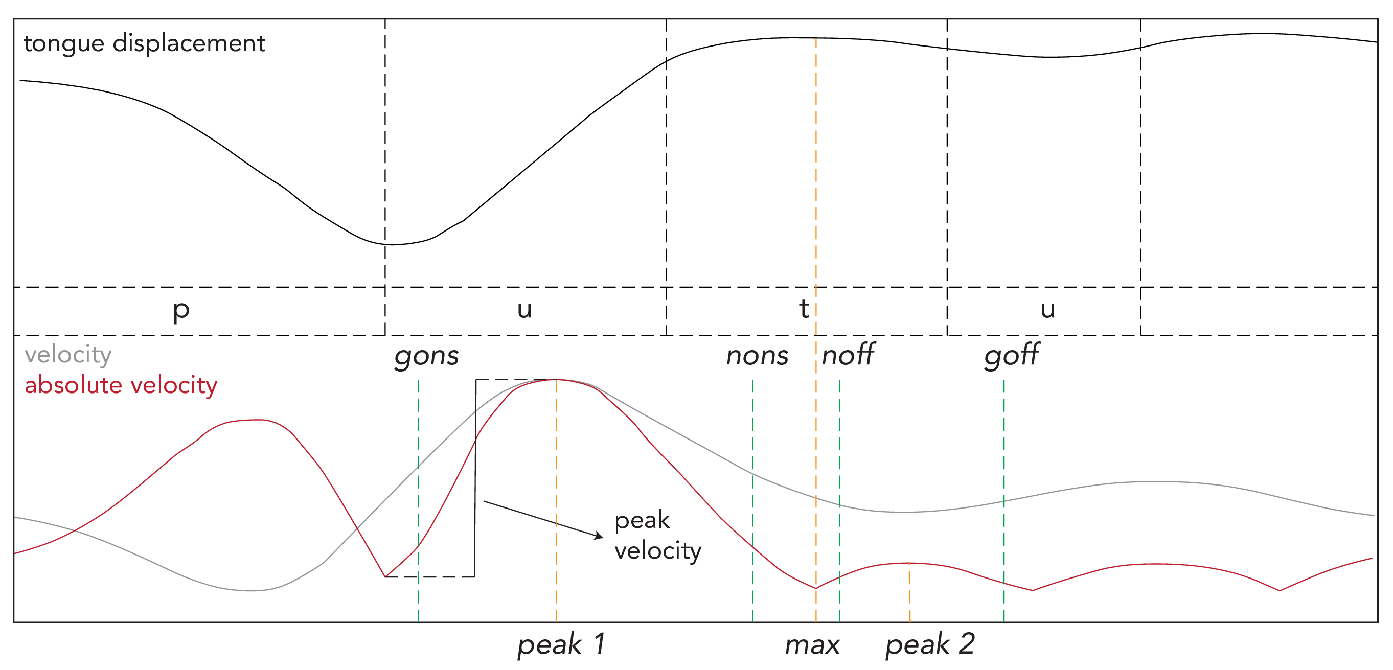
Figure 3.4: Gestural landmarks of tongue movements in the word putu. The top panel shows tongue tip displacement, while the bottom panel shows tangential and absolute velocity.
The Cartesian coordinates of the fitted splines, together with tongue displacement, tangential velocity, and absolute velocity of the tongue root, dorsum and tip, were obtained at the times corresponding to the following gestural landmarks: C2 closure onset, tongue maximum displacement during C2 closure (MAX), peak absolute velocity before and after tongue maximum displacement (PEAK_1 and PEAK_2), tongue closing gesture onset (GONS), closing gesture nucleus onset (NONS) and offset (NOFF). Tongue displacement, and the tangential and absolute velocities of the tongue root, dorsum, and tip were also extracted as time-series along the entire duration of V1. The coordinates of the splines were converted from Cartesian to polar for statistical analysis (see A). As discussed in 2.1, Study I set out to gather data on acoustic segmental durations, the timing of the consonantal gestures, and properties of vocal fold vibration. For this reason, tongue movement velocity was not analysed as part of the current investigation, and future work on this aspect is warranted.
Finally, wavegram data was extracted from the EGG data, following the method proposed by Herbst, Fitch & Švec (2010). In brief, a wavegram is a spectrogram-like representation of the EGG signal, where individual glottal cycles are sequentially placed on the x-axis, the normalised time of the samples taken from within each glottal cycle is the y-axis, and the third dimension, represented by colours of different shading, is the normalised amplitude of the EGG signal. Wavegram data was obtained from the entire duration of V1. See 7 for the detailed procedure.
3.2 Compensatory aspects of the effect of voicing on vowel duration in English (Study II)
The results from Study I indicated that the temporal distance between two consecutive stop releases in disyllabic words of Italian and Polish is not affected by the voicing of the second stop (4). Within this temporally stable interval, differences in the timing of oral closure determines the respective durations of the vowel and the consonant closure. Thus, a second study was carried out to assess whether the durational pattern found in Study I would generalise to English, and to investigate differences between disyllabic and monosyllabic words as predicted by a word-holistic account of gestural phasing (5). It was expected that, while the duration of the release-to-release interval would be insensitive to the voicing status of the second consonant, the interval would be longer in monosyllabic words with a voiced consonant. 5 discusses the empirical and theoretical foundation of the research hypotheses and methods of Study II more in detail. A brief synthesis of the methodologies of the study is reported here.
Fifteen university students were recorded in a sound attenuated room in the Phonetics Laboratory of the University of Manchester while reading sentence stimuli containing test words, presented on a computer screen with PsychoPy (Peirce 2009).
The participants were native speakers of British English, aged between 20 and 29, born and raised within Greater Manchester.7
The test words were built according to the following structure: CV́C(VC), where C = /t/, V = /iː, ɜː, ɑː/, C = /p, b, k, g/, and (VC) = /əs/.
The issue of the syllabification of word-medial consonants in English is far from settled and still a controversial topic in English phonology.
All possible syllabification options continue to be defended (Bermúdez-Otero 2013): onset-maximal syllabification, rhyme-maximal
syllabification, and ambisyllabicity.
Bermúdez-Otero (2013) offers initial phonological evidence for preferring an onset-maximal approach.
This view is adopted as a working assumption in this work, and C2 in CVCV words are taken to be onsets.
Future articulatory work is needed to shed light on the syllabification issue.
The target words were embedded within five different frame sentences, so that each speaker would read a total of 120 stimuli (24 words × 5 frames).
The audio recordings were force-aligned and the times of acoustic landmarks were extracted according to the same procedure as in Study I (with make-textgrid.praat and get-measurements.praat in Coretta 2019a).
3.3 Open Science
Open Science is a movement that stresses the importance of a more honest and transparent scientific attitude by promoting a series of research principles and by warning from common, although not necessarily intentional, questionable practices and misconceptions. The term Open Science as a whole refers to the fundamental concepts of “openness, transparency, rigour, reproducibility, replicability, and accumulation of knowledge” (Crüwell et al. 2018: 3). The goodness of the latter depends in great part on the reproducibility and replicability of the studies that contribute to knowledge accumulation. While the terms “reproducibility” and “replicability” are generally used interchangeably, they refer to two different ideas. A study is replicable when researchers can independently run the study on new subjects/data and obtain the same results (in brief, same analysis, different data/researchers). The reproducibility of a study is, instead, related to the ability of independent researchers to run the original analysis on the original data and obtain the same results as those presented by the original authors, pending enough information on the analysis procedures is given (in brief, same analysis, same data).
A sense of need for Open Science, now increasingly spreading to different disciplines and enterprises, arose primarily from the ongoing so-called “replication crisis” (Pashler & Wagenmakers 2012; Schooler 2014), which has attracted the most attention within the circles of medical and psychological sciences. Recent attempts to replicate results from high-impact studies in psychology have demonstrated an alarmingly high rate of failure to replicate. For example, in a replication attempt of 100 psychology studies, only 39% of the original results were rated by annotators as successfully replicated (Open Science Collaboration 2015). Failure to replicate previous results have been claimed to be a consequence of low statistical power (Button et al. 2013), and of so-called questionable research and measurement practices (Simmons, Nelson & Simonsohn 2011; Morin 2015; Flake & Fried 2019). The following sections discuss these problems in turn.
3.3.1 “With great power comes great replicability”
One of the issues that can affect statistical analysis is related to errors in rejecting the null hypothesis.8 A researcher could falsely reject the null hypothesis when in fact is correct (Type I errors, an effect is found when there is none), or they could falsely fail to reject the null hypothesis when in fact it should have been (Type II errors, an effect is not found when there is one). Type I and Type II errors do occur and cannot be totally prevented. Rather, the aim is to keep their rate of occurrence as low as possible. The generally accepted rates of Type I and Type II errors are 0.05 and 0.2 respectively (usually referred to as the \(\alpha\) and \(\beta\) levels). This means that, in a series of imaginary multiple replications of a study, 5% of the times the null hypothesis will be falsely rejected, and 20% of the times will falsely be not rejected. A concept closely related to Type II errors is statistical power, which is the probability of correctly rejecting the null hypothesis when it is false (calculated as \(B = 1 - \beta\)). In other words, power is the probability of detecting an effect equal or greater than a specified effect size. Given the standard \(\beta = 0.2\), an accepted (minimum) power threshold is 80% (which means that an effect equal or greater than a chosen size will be detected 80% of the time).
Two other types of statistical errors are the Type S (sign) and Type M (magnitude) errors (Gelman & Tuerlinckx 2000; Gelman & Carlin 2014). Type S errors refer to the probability of the estimated effect having the wrong sign (for example, finding a positive effect when in reality the effect is negative), while Type M errors correspond to the exaggeration ratio (the ratio between the estimated and the real effect). When the statistical power of a study is low (below 50%), Gelman & Carlin (2014) show that the exaggeration ratio (Type M error) is particularly high (from 2.5 up to 10 times the true effect size). Type S errors (wrong sign) are more common at lower power levels (below 10%), although these can easily arise due to small sample sizes and high variance.
Several researchers have shown that the average statistical power of studies in different disciplines is very low (35% or below) and that the last 50 years did not witness an improvement. Bakker, Dijk & Wicherts (2012) show that the median statistical power in psychology is 35%, while Button et al. (2013) reports a median of 21% obtained from 48 neuroscience meta-analyses. In Dumas-Mallet et al. (2017), half of the surveyed biomedical studies (N = 660) have power below 20%, while the median ranges between 9% and 30% depending on the subfield. Rossi (1990) and Marszalek et al. (2011) show that from the 70s to date there hasn’t been an increase in power and sample sizes. Tressoldi & Giofré (2015) also find that only 2.9% of 853 studies in psychology report a prospective power analysis for sample size determination, i.e. the estimation of the smallest sample size necessary to obtain a certain power level before the experiment is run. In sum, low statistical power (well below the recommended 80% threshold) seems to be the norm.
3.3.2 The dark side of research
Questionable research and measurement practices are practices that negatively affect the scientific enterprise, but that are employed (most of the time unintentionally) by a surprisingly high number of researchers (John, Loewenstein & Prelec 2012). Silberzahn et al. (2018) asked 29 teams (61 analysts) to answer the same research question given the same data set, and showed that data analysis can be highly subjective. A total of 21 unique combinations of predictors were used across the 29 teams, leading to diverging results (20 teams obtained a significant result, while 9 did not). At various stages of the study timeline, a researcher can exploit the so-called “researcher’s degrees of freedom” to obtain a significant result (Simmons, Nelson & Simonsohn 2011). The researcher’s degrees of freedom create a “garden of forking paths” (Gelman & Loken 2013), that the researcher can explore until the results are satisfactory (i.e., they lead to high-impact or expected findings).
P-hacking is a general term that refers to the process of choosing and reporting those analyses that change a non-significant p-value to a significant one Wagenmakers (2007). P-hacking can be achieved by several means, for example by trying different dependent variables, including and/or excluding predictors, selective inclusion/exclusion of subjects and observations, or sequential testing (collecting data until the results are significant). Another common practice is to back-engineer a hypothesis after obtaining unexpected results, also known as Hypothesising After the Results are Known (HARKing, Kerr 1998). Lieber (2009) warns against “double dipping,” or the use of the same data to generate a hypothesis and test it. Morin (2015) and Flake & Fried (2019) more specifically discuss questionable practices related to how research variables are measured and operationalised. The literature reviewed in Flake & Fried (2019) suggests that a very high percentage of published papers contains measures that are created on the fly but lack any reference to reliability tests. Researchers have also been found to manipulate validated scales to obtain desired results.
Cognitive biases and statistical misconceptions can also have a negative impact on research conduct. Wagenmakers et al. (2012) discuss the effects of cognitive biases like the confirmation bias (the tendency to look for facts and interpretations that confirm one’s prior conviction, Nickerson 1998) and the hindsight bias (the tendency to find an event less surprising after it has occurred, Roese & Vohs 2012). Greenland (2017) defines further common distortions pertaining to methodological approaches, like statistical reification (interpreting statistical results as reflections of an actual physical reality). Finally, Wagenmakers (2007) and Motulsky (2014) examine mistaken beliefs about the meaning of p-values and statistical significance (like interpreting p-values as an index to statistical evidence or the idea that p-values inform us about the likelihood of the null-hypothesis given the data).
A bias in the observed effects can also arise at the stage of publication. A publication bias has been observed in that significant and novel results are generally favoured over null results or replications (Easterbrook et al. 1991; Ioannidis 2005; Song et al. 2010; Kicinski 2013; Nissen et al. 2016). Rosenthal (1979) called the bias against publishing null results the “file drawer” problem. Studies that don’t lead to a significant result are stored in a metaphorical file drawer and forgotten. This practice not only can bias meta-analytical effect sizes, but also allows for waste of resources when studies with undisclosed null results are repeatedly performed. The questionable research and measurement practices described above, together with publication bias, conspire to unduly increase confidence in our research outcomes. A final exculpatory note is due, though, in that these practices are not necessarily intentional or fraudulent, and in some cases lie within a “grey area” of accepted standard procedures.
3.3.3 Where we stand and where we are heading
Given the similarities in methods between the psychological sciences and phonetics/phonology, it is reasonable to assume that the situation does not fare better in the latter. As mentioned above, sample size, coupled with the effects of increased variance due to between-subject designs, can have a big impact on statistical power. Kirby & Sonderegger (2018) suggest that the number of participants in phonetic studies is generally low, and that, even with nominally high-powered sample sizes, estimation of small effect sizes is subject to the power-related issues discussed above (especially Type S/M errors). Nicenboim, Roettger & Vasishth (2018) further show how low statistical power has adverse effects on the investigation of phonetic phenomena characterised by small effect sizes, like incomplete neutralisation. Winter (2015) further argues that the common practice of using few items (e.g. word types) and a high number of repetitions increases statistical certainty of the estimates of idiosyncratic differences between items rather than those of the sought effects. Roettger (2019) discusses how the inherently multidimensional nature of speech favours exploration of the researcher’s degrees of freedom, by allowing the researcher to navigate through a variety of choices of phonetic correlates and their operationalisation.
In a review of 113 studies of acoustic correlates of word stress in a variety of languages, published between 1955 and 2017, Roettger & Gordon (2017) show that the majority of studies include 1 to 10 speakers (mode = 1), 1 to 40 lexical items, and 1 to 6 repetitions. A follow-up analysis conducted on the same data indicates that the median number of participants per study is 5 (see E). A few recent studies (2010 onwards) constitute a clear exception by having more than 30 participants. However, no apparent trend of increasing average number of speakers can be observed and the situation has been fairly stable over the years. Finally, the language endangerment status has a small but negligible negative effect on participants’ number in vulnerable and definitely endangered languages, but not so much in severely and critically endangered ones. It is reasonable to assume that, based on this cursory analysis, sample size in phonetic studies is generally very low, independent from publication year and endangerment status.
As a partial remedy to the issues discussed so far, researchers have proposed two solutions: pre-registrations and Registered Reports. Pre-registration of a study consists in the researchers’ commitment to an experimental and analytical protocol before collecting and seeing the data (Wagenmakers et al. 2012; Veer & Giner-Sorolla 2016). Pre-registering a study establishes a clear separation between confirmatory (hypothesis-testing) analyses and exploratory (hypothesis-generating) research. While both types of research are essential to scientific progress (Tukey 1980), presenting exploratory analyses as confirmatory is detrimental to it. Pre-registrations ensure researchers comply to such demarcation, while leaving space to generate new hypotheses via exploratory research. A more recent initiative proposes Registered Reports as a publication format that can counteract questionable research practices and the exploitation of the researcher’s degrees of freedom (Chambers et al. 2015). At the time of writing, no journal specialised in phonetics/phonology offers this article format, although it is currently under implementation at the Journal of the Association for Laboratory Phonology and a few other journals focussed on other linguistic fields.9
Another incentive to developing a transparent research attitude comes from aspects of reproducibility. As discussed above, a research analysis is reproducible when different researchers obtain the same results as in the published study by running the same analysis on the same data. Ensuring full reproducibility also means ensuring computational reproducibility, or in other words enabling researchers to perform the original analysis in an identical computational environment (Schwab, Karrenbach & Claerbout 2000; Fomel & Claerbout 2009). Peng (2009) mentions exposed cases of fraudulent data manipulation and unintentional analysis errors that call for policies of reproducibility to ensure accountability of published results. Our field is not immune from these issues (see for example the “Yokuts vowels” case, Weigel 2002; Weigel 2005; Blevins 2004), and the idea of reproducibility is not new to linguistics in general (Bird & Simons 2003; Thieberger 2004; Maxwell & Amith 2005; Maxwell 2013; Cysouw 2015; Gawne et al. 2017) nor to phonetics/phonology specifically (Abari 2012; Roettger 2019).
The objective of making research accountable can be achieved by publicly sharing data (subject to ethical restrictions), analysis code, and detailed information on the software that produced the results (Sandve et al. 2013). Sharing data is also fundamental for the accumulation of knowledge, for example in the context of meta-analytical studies. Several services are now available which offer free online data storage and versioning, like the Open Science Framework, GitHub, and DataHub. Extensive documentation of code takes on an important role, and the paradigm of literate programming offers a practical solution (Knuth 1984). Within the literate programming framework, code and documentation coexist within a single source file, and code snippets are interweaved with their documentation. Reproducible reporting further implements this concept (Peng 2015) by automating the generation and inclusion of summary tables, statistics, and figures in a paper using statistical software like R (R Core Team 2019). In a reproducible report, data and results are computationally linked via the statistical software, and changes in data or analyses are reflected in changes in the results appearing in the text. This workflow reduces chances of reporting errors and facilitates validation of the data analyses by other researchers.
3.3.4 Putting this into practice
The research project behind this dissertation has been carried out with principles of Open Science in mind. The reader might notice, however, a certain arc of development in putting these concepts into practice, since my understanding of Open Science practices evolved during the realisation of the project. This last section of the Introduction discusses how the principles and methods expounded in the above sections were applied in this project.
Study I was not pre-registered, since the absence of a specific hypothesis did not allow for the formulation of a corresponding analysis. Sample size was determined on the basis of practical considerations concerning the time required for processing ultrasound tongue imaging data. Several different parameters and models have been explored in search of relevant patterns, while only a few of these have been reported in the papers of this study. The models of Study I were conducted within a Neyman-Pearson (frequentist) framework of statistical inference (Perezgonzalez 2015), while a Bayes factor analysis (Kass & Raftery 1995) was performed in those cases that demanded it (4). To compensate for the asymmetry between the number of models run and those reported, less attention has been given to p-values, while greater focus was placed on effect sizes and their hypothesis-generating value. The design and analyses of Study II were pre-registered on the Open Science Framework (https://osf.io/2m39u/). Sample size determination followed the method of the Region Of Practical Equivalence (Vasishth, Mertzen, et al. 2018). Data from Study II was subject to a full Bayesian analysis, and greater emphasis was given on the posterior probability distributions of the effect estimates rather than on their means (5).
Data, code, and information about software can be found in the research compendium of this project on the Open Science Framework (Coretta 2020: https://osf.io/w92me/). This OSF repository acts as a hub for the research compendia of the project and of the individual papers. The data has been packaged and documented using R (Marwick, Boettiger & Mullen 2017). The data packages (coretta2018itapol and coretta2019eng) are available on GitHub and links to them are given in the OSF repository (see the Data components in the repository). Following the recommendations in Berez-Kroeker et al. (2018), each data component is given a standard bibliographical citation (Coretta 2018a; Coretta 2019a).
Data processing using Praat scripting followed the principles of literate programming, i.e. code and documentation coexist in a single source file. The source files were written in literate markdown, a flavour of markdown that allows extracting code from markdown text to build the scripts from the source file. The scripts were extracted from the literate source file using the Literate Markdown Tangle software10 and were run with a custom R package, speakr (Coretta 2019b). The documentation of the scripts was generated with Pandoc11 and a custom Praat syntax highlighting extension (available in speakr). All analyses and derived figures in this dissertation can be reproduced in R (R Core Team 2019) with the scripts found in the papers’ respective compendia.
The following software and packages were used: tidyverse (Wickham 2017), lme4 (Bates et al. 2015), lmerTest (Kuznetsova, Bruun Brockhoff & Haubo Bojesen Christensen 2017), effects (Fox & Weisberg 2019), broom.mixed (Bolker & Robinson 2019), mgcv (Wood 2017), itsadug (van Rij et al. 2017), Stan (Stan Development Team 2017), brms (Bürkner 2017), tidybayes (Kay 2019). I developed two R packages for the visualisation of generalised additive models using tidyverse software (tidymv, Coretta 2019c) and the analysis of ultrasound tongue imaging data with mgcv (rticulate, Coretta 2018b). This dissertation was written in R Markdown, and typeset with knitr and bookdown (Xie 2014; Xie 2016; Xie, Allaire & Grolemund 2018; Xie 2019).
No sociolinguistic information was collected for this study, given that sociolinguistic considerations were not part of the study aims and given the sensitivity of the data.↩︎
The quote in the title is from a 2016 twitter status by Nathan C. Hall (https://twitter.com/prof_nch/status/790744443313852417?s=20).↩︎
See the spreadsheet at this link for a curated list: https://docs.google.com/spreadsheets/d/17dLaqKXcjyWk1thG8y5C3_fHXXNEqQMcGWDY62BOc0Q/edit?usp=sharing.↩︎