Code
library(tidyverse)
theme_set(theme_light())
library(brms)
library(posterior)
library(ggdist)This study sets out to answer the following questions:
Does the lexical status of the word affect reaction times?
Does the mean phone-level Levenshtein distance affect reaction times?
Does the effect of mean phone-level distance on reaction times differ depending on the lexical status?
library(tidyverse)
theme_set(theme_light())
library(brms)
library(posterior)
library(ggdist)In order to answer the research questions presented in Section 1, we fitted a Bayesian regression model with brms (Bürkner 2017, 2018) in R version 4.5.0 (R Core Team 2025). The model was first run with four MCMC chains and 2000 iterations, of which 1000 for warm-up. Since the resulting estimated sample size (ESS) was flagged by brms as too low, we refitted the model by increasing the number of iterations to 4000 (of which 2000 for warm-up). The model fully converged with \(\hat{R}\) values of approximately 1 and sufficient ESS.
mald <- readRDS("data/mald.rds") |>
  mutate(
    PhonLev_c = PhonLev - mean(PhonLev)
  )

# Model with iter = 2000 gave warning of low ESS. Fit with iter = 4000.

rt_full <- brm(
  RT ~ 0 + IsWord + IsWord:PhonLev_c +
    (0 + IsWord + IsWord:PhonLev_c | Subject),
  family = lognormal,
  data = mald,
  cores = 4,
  iter = 4000,
  seed = 7238,
  file = "data/cache/rt_full.rds"
)
The model structure was the following: we used a log-normal distribution for the outcome variable, i.e. the reaction times (RTs). A log-normal distribution is a standard distribution for numeric variables that are bounded to positive values only, like reaction times (see e.g. Rosen 2005). We included the following predictors: lexical status of the target word (real vs nonce) and mean phone-level Levenshtein distance of the target word (range approx. 5-14). The lexical status predictor was coded using indexing rather than traditional contrasts (McElreath 2019) by suppressing the model’s intercept with the 0 + syntax in the model’s formula. The mean phone-level distance was centered by subtracting the grand mean of the mean phone-level distance. An interaction between lexical status and phone-level distance was also included. Furthermore, we included varying terms (aka random terms, see Gelman 2005) by subject for lexical status, phone-level distance and the interaction between the two. We did not include by-word varying terms since the majority of data is from distinct words (the exceptions are 130 words of 2867 which have two or three observations in total, rather than one). We used the brms default priors. Table 1 reports the mean, standard deviation and lower and upper limits of the 95% Credible Interval (CrI) for the model’s coefficients in logs and log-odds (which is the scale returned by log-normal regressions). For ease of interpretation, we will also convert estimands to odds and milliseconds where relevant.
fixef(rt_full) |>
  as_tibble(rownames = "coefficient") |>
  rename(mean = Estimate, SD = Est.Error, lower = Q2.5, upper = Q97.5) |>
knitr::kable(digits = 2)| coefficient | mean | SD | lower | upper |
|---|---|---|---|---|
| IsWordTRUE | 6.85 | 0.02 | 6.82 | 6.88 |
| IsWordFALSE | 6.97 | 0.02 | 6.92 | 7.01 |
| IsWordTRUE:PhonLev_c | 0.03 | 0.01 | 0.02 | 0.04 |
| IsWordFALSE:PhonLev_c | 0.02 | 0.01 | 0.01 | 0.03 |
rt_full_draws <- as_draws_df(rt_full) |>
  mutate(
    isword_diff = exp(`b_IsWordFALSE`) - exp(`b_IsWordTRUE`),
    dist_diff = `b_IsWordFALSE:PhonLev_c` - `b_IsWordTRUE:PhonLev_c`
  )

round(quantile2(rt_full_draws$isword_diff))
Starting with RQ1, according to the model, the mean RT with real words (IsWordTRUE), when the mean phone-level distance is at its grand mean (approx 7), is between 916 and 973 ms, at 95% probability. With nonce words (IsWordFalse) and average mean phone-level distance, the mean RT is between 1012 and 1108 ms, at 95% probability. The estimated difference in RT between nonce vs real words at average phone-level distance is between 84 and 152 ms, at 95% confidence. Such difference can be regarded as cognitively relevant and related to delays in processing of nonce words due to their absence in the mental lexicon (Luce and Pisoni 1998; Luce and McLennan 2005; Pisoni et al. 1985). Note that, given the nature of the log-normal distribution, the difference in milliseconds is smaller with smaller phone-level distance and greater with greater phone-level distance. This is true independent of whether the phone-level distance effect is the same or different in real and nonce words. Figure 1 shows the predicted reaction times depending on (centred) phone-level distance and lexical status.
conditional_effects(rt_full, "PhonLev_c:IsWord")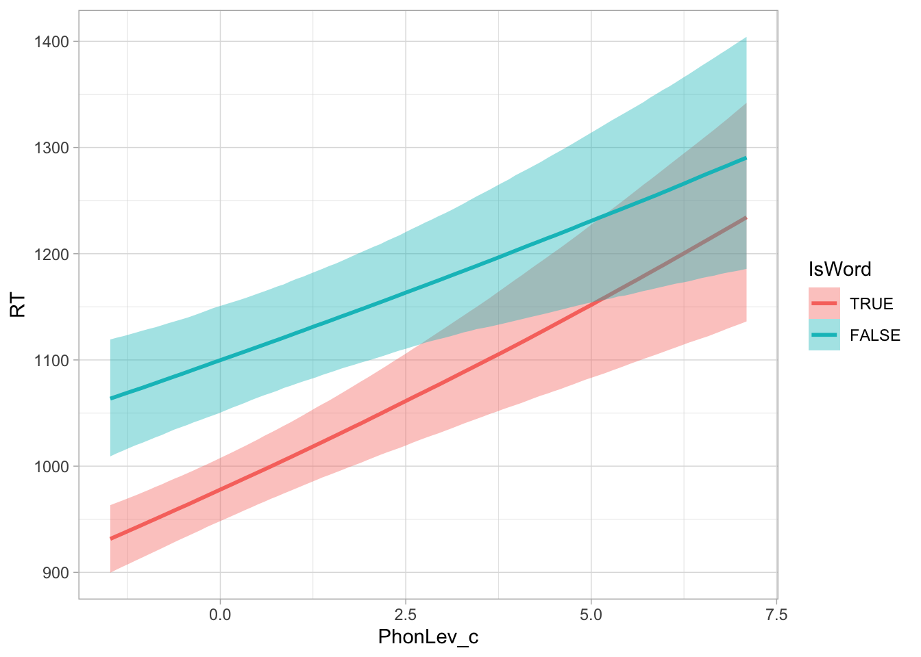
# Calculate odds-ratio for real words
round(exp(c(0.02, 0.04)), 2)
# Calculate odds-ratio for nonce words
round(exp(c(0.01, 0.03)), 2)
# Calculate odds-ratio between distance = 5 vs 14 (real words)
round(exp(c(0.02*9, 0.04*9)), 2)
# Calculate odds-ratio between distance = 5 vs 14 (odd words)
round(exp(c(0.01*9, 0.03*9)), 2)
Moving onto the effect of mean phone-level distance (RQ2), the model suggest an appreciable increase in RTs with greater phone-level distance: the estimated effect for each unit increase in distance is an increase of 0.02-0.04 log-ms (2-4% increase) with real words and an increase of 0.01-0.03 log-ms (1-3% increase) with nonce words. The phone-level distance in the data ranges from about 5 to about 14 (mean = 7). When comparing real words with distance = 5 to real words with distance = 14, we can expect an average increase of about 20-40% (at 95% confidence). For nonce words, the increase is between 9-31% (at 95% confidence). We interpret these estimates to indicate a moderately robust effect of distance in both real and nonce words.
round(quantile2(rt_full_draws$dist_diff), 3)
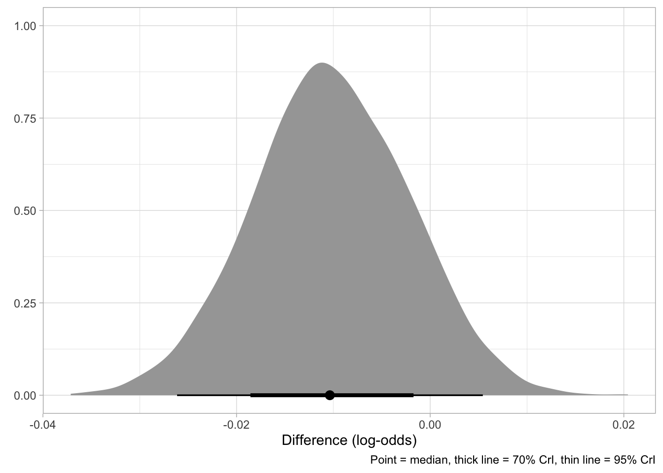
round(quantile2(rt_full_draws$dist_diff, c(0.15, 0.85)), 3)As to the question of whether the effect of phone-level distance is different in real vs nonce words (RQ3), the 95% CrI of the difference is [-0.024, +0.003], spanning both negative and positive values, with an appreciable skew towards negative values. The density of the posterior distribution of the difference is shown in Figure 2. The median, 70% and 95% CrI are represented by the dot, the thick and think lines respectively at the bottom of the density. The 70% CrI of the difference is [-0.019, -0.002] which spans negative values only. This indicates that we can be 70% confident that the difference in phone-level distance effect between nonce and real words is possibly negative, albeit with uncertain magnitude (i.e. the difference could be quite small if not negligible).
rt_full_draws |>
  ggplot(aes(dist_diff)) +
  stat_halfeye(.width = c(0.70, 0.95)) +
  labs(
    x = "Difference (log-odds)", y = element_blank(),
    caption = "Point = median, thick line = 70% CrI, thin line = 95% CrI"
  )
phonlev_diff_5_10 <- rt_full_draws |>
  mutate(
    true_5 = exp(b_IsWordTRUE - `b_IsWordTRUE:PhonLev_c` * 2),
    false_5 = exp(b_IsWordFALSE + `b_IsWordFALSE:PhonLev_c` * 2),
    true_10 = exp(b_IsWordTRUE + `b_IsWordTRUE:PhonLev_c` * 3),
    false_10 = exp(b_IsWordFALSE + `b_IsWordFALSE:PhonLev_c` * 3),
    ft_5 = false_5 - true_5,
    ft_10 = false_10 - true_10,
    ft_10_5 = ft_10 - ft_5
  ) |>
  select(ft_5, ft_10, ft_10_5)

round(quantile2(phonlev_diff_5_10$ft_5))
round(quantile2(phonlev_diff_5_10$ft_10))
round(quantile2(phonlev_diff_5_10$ft_10_5))

phonlev_diff_5_10_mean <- rt_full_draws |>
  mutate(
    mean_PhonLev = mean(c(`b_IsWordTRUE:PhonLev_c`, `b_IsWordFALSE:PhonLev_c`)),
    true_5 = exp(b_IsWordTRUE - mean_PhonLev * 2),
    false_5 = exp(b_IsWordFALSE + mean_PhonLev * 2),
    true_10 = exp(b_IsWordTRUE + mean_PhonLev * 3),
    false_10 = exp(b_IsWordFALSE + mean_PhonLev * 3),
    ft_5 = false_5 - true_5,
    ft_10 = false_10 - true_10,
    ft_10_5 = ft_10 - ft_5
  ) |>
  select(ft_5, ft_10, ft_10_5)

round(quantile2(phonlev_diff_5_10_mean$ft_5))
round(quantile2(phonlev_diff_5_10_mean$ft_10))
round(quantile2(phonlev_diff_5_10_mean$ft_10_5))
To illustrate what the difference in phone-level distance effect would look like in milliseconds, we calculated the 95% CrI of the difference in RTs between nonce and real words with phone-level distance = 5 vs with distance = 10. When the phone-level distance is 5, the 95% CrI (of the difference in RTs between nonce and real words) is [+187, +267] ms, while when the phone-level distance is 10 the 95% CrI is [+42, +148]. Now let’s compare these 95% CrIs with CrIs calculated assuming the same effect of phone-level distance in real and nonce words (i.e. by using the mean of the phone-level distance effect in real and nonce words): the 95% CrI with distance = 5 is [+194, +265] ms while the 95% CrI with distance =10 is [+92, +165] ms. The comparison suggests that, if indeed there is a difference in the effect of phone-level distance between real and nonce words with magnitudes as suggested by the model, we would get an appreciable effect in the difference between real and nonce words depending on the phone-level distance, by which with higher phone-level distances the gap in RTs between nonce and real words would diminish. We find this to be theoretically relevant, but given the uncertainty in the estimated difference in phone-level distance effect, we leave this to future work.
To summarise, we find an appreciable difference in reaction times between real and nonce words, especially at lower phone-level distance. The phone-level distance has a positive effect on reaction times, with longer reaction times when the distance is higher. Possibly, the positive effect of the distance on reaction times is weaker in nonce words, meaning that the difference in reaction time between real and nonce words might decrease with increasing phone-level distance.