Introduction to Bayesian regression models

03 - Diagnostics

Stefano Coretta

University of Edinburgh

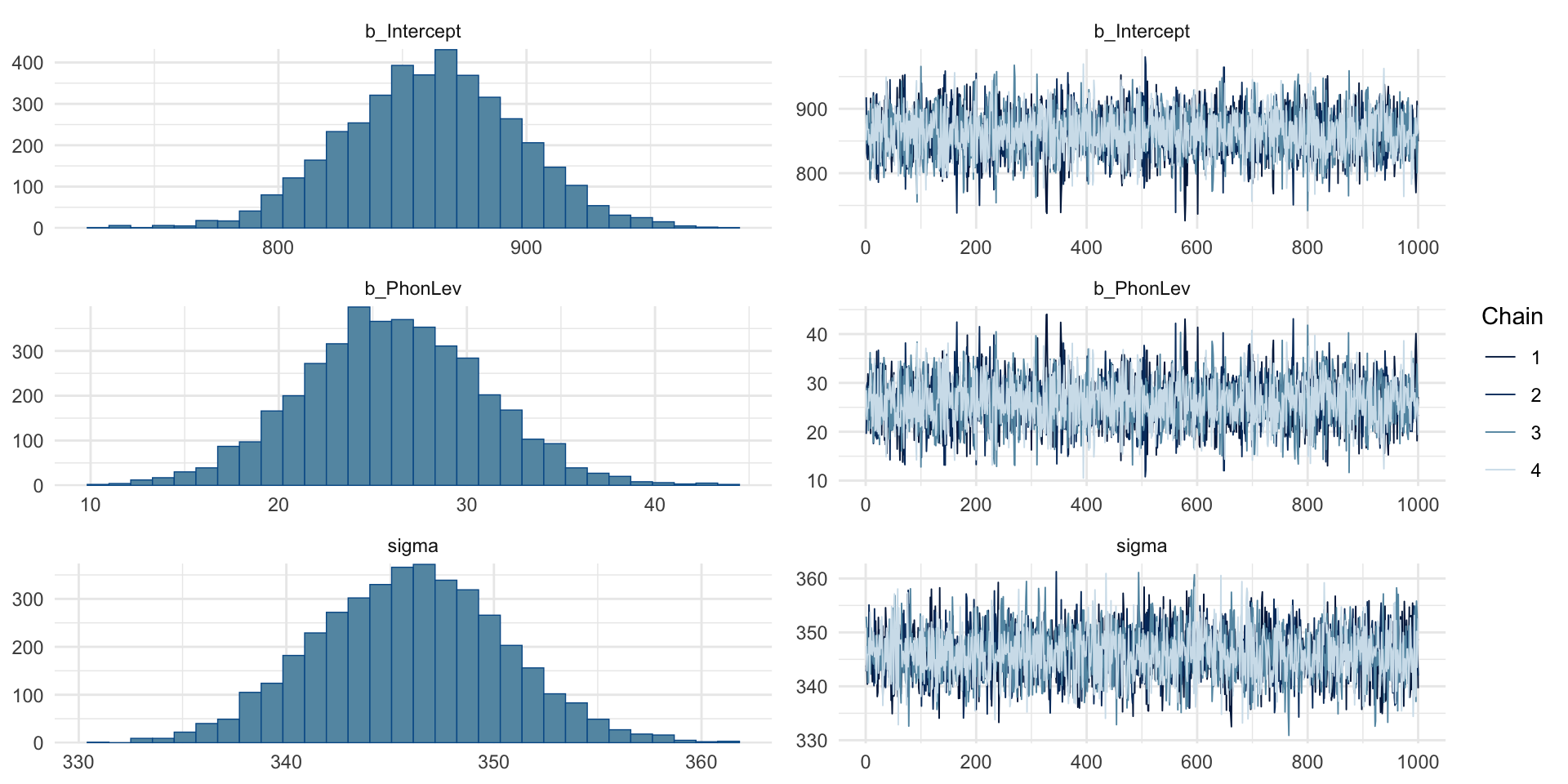
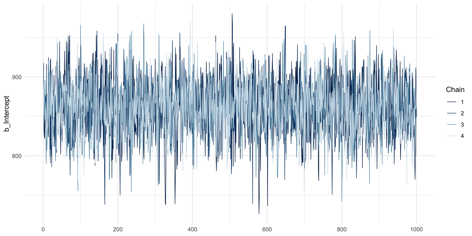
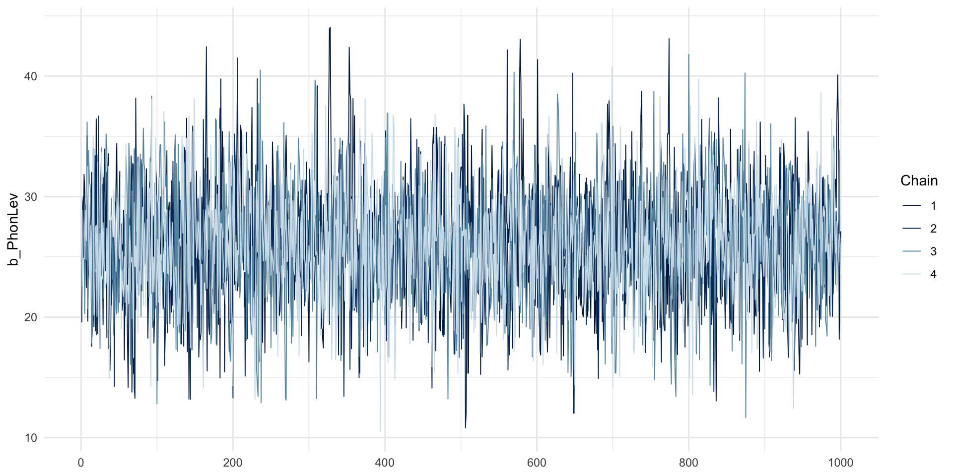
MCMC traces

plot(brm_lev)

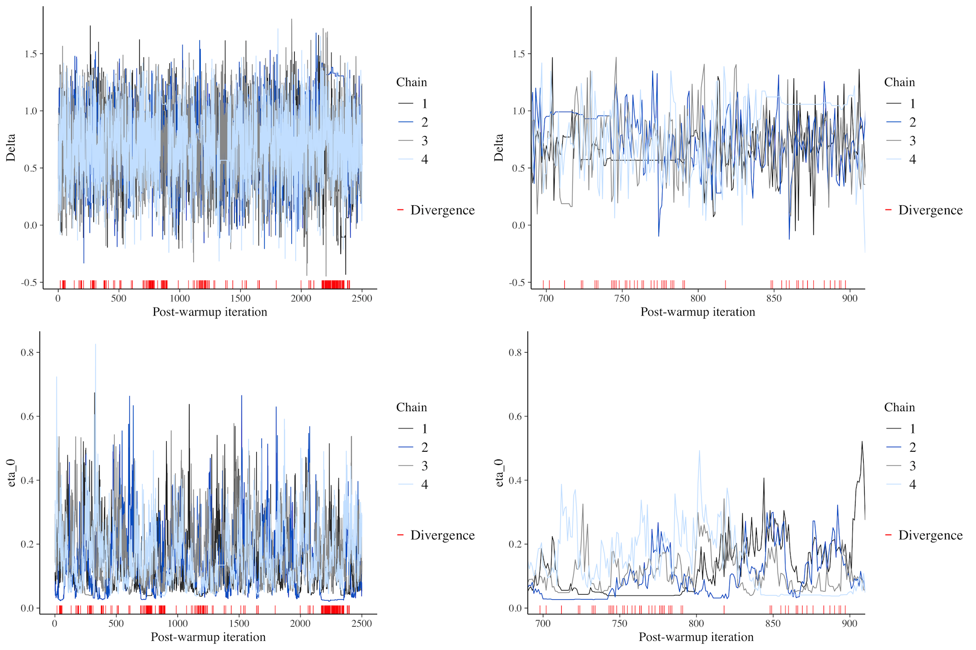
MCMC traces: bad

An example of bad MCMC chain mixing.

MCMC traces: intercept

as.array(brm_lev) %>%
  mcmc_trace("b_Intercept", np = nuts_params(brm_lev))

MCMC traces: `IsWord`

as.array(brm_lev) %>%
  mcmc_trace("b_PhonLev", np = nuts_params(brm_lev))

\(\hat{R}\) and Effective Sample Size (ESS)

brm_lev

 Family: gaussian 
  Links: mu = identity; sigma = identity 
Formula: RT ~ 1 + PhonLev 
   Data: mald (Number of observations: 3000) 
  Draws: 4 chains, each with iter = 2000; warmup = 1000; thin = 1;
         total post-warmup draws = 4000

Regression Coefficients:
          Estimate Est.Error l-95% CI u-95% CI Rhat Bulk_ESS Tail_ESS
Intercept   861.62     35.11   793.25   929.05 1.00     4139     2815
PhonLev      26.05      4.85    16.70    35.40 1.00     4169     2866

Further Distributional Parameters:
      Estimate Est.Error l-95% CI u-95% CI Rhat Bulk_ESS Tail_ESS
sigma   345.95      4.54   337.09   354.71 1.00     3849     2919

Draws were sampled using sampling(NUTS). For each parameter, Bulk_ESS
and Tail_ESS are effective sample size measures, and Rhat is the potential
scale reduction factor on split chains (at convergence, Rhat = 1).

brms warns you

What to do

Increase the number of iterations (default is 2000): iter = 4000.
Increase adapt_delta (an MCMC setting, default is 0.9, can only be between 0 and 1 exclusive).
- control = list(adapt_delta = 0.9999)
Increase max_treedepth (another MCMC settings, default is 10).
- control = list(max_treedepth = 15)

These solutions increase the time needed to fit the model, which is a perfectly acceptable compromise.

Fictitious example

mod <- brm(
  y ~ x,
  data = dat,
  iter = 4000,
  control = list(adapt_delta = 0.9999, max_treedepth = 15)
)

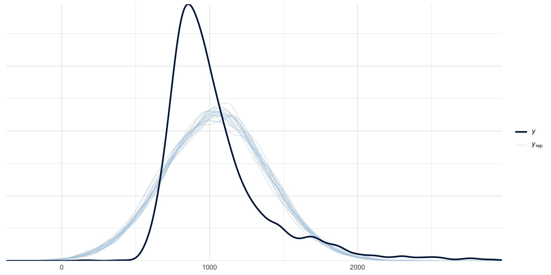
Posterior Predictive Checks

pp_check(brm_lev, ndraws = 20)

Log-normal regression

\[ \begin{align} RT & \sim Lognormal(\mu, \sigma)\\ log(\mu) & = \beta_0 + \beta_1 \cdot \text{PhonLev}\\ \end{align} \]

Variables that can only be positive, like Reaction Times, cannot be Gaussian.
A standard distribution for these variables is the log-normal distribution.

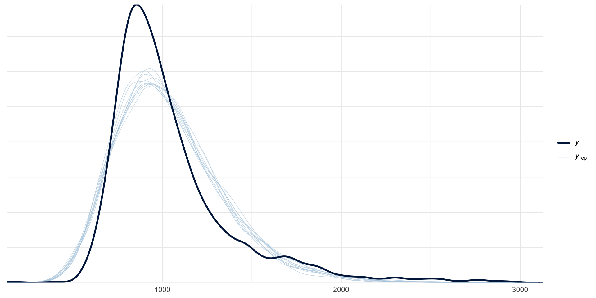
Log-normal regression: MALD

mald <- readRDS("./data/mald.rds")

brm_log <- brm(
  RT ~ 1 + PhonLev,
  data = mald,
  family = lognormal,
  cores = 4,
  seed = 9812,
  file = "data/cache/brm_log.rds"
)

Log-normal regression: summary

brm_log

 Family: lognormal 
  Links: mu = identity; sigma = identity 
Formula: RT ~ 1 + PhonLev 
   Data: mald (Number of observations: 3000) 
  Draws: 4 chains, each with iter = 2000; warmup = 1000; thin = 1;
         total post-warmup draws = 4000

Regression Coefficients:
          Estimate Est.Error l-95% CI u-95% CI Rhat Bulk_ESS Tail_ESS
Intercept     6.71      0.03     6.66     6.76 1.00     4948     3345
PhonLev       0.03      0.00     0.02     0.04 1.00     4954     3380

Further Distributional Parameters:
      Estimate Est.Error l-95% CI u-95% CI Rhat Bulk_ESS Tail_ESS
sigma     0.28      0.00     0.28     0.29 1.00     2395     2781

Draws were sampled using sampling(NUTS). For each parameter, Bulk_ESS
and Tail_ESS are effective sample size measures, and Rhat is the potential
scale reduction factor on split chains (at convergence, Rhat = 1).

Posterior Predictive Checks: looks better!

pp_check(brm_log, ndraws = 10)

Predicted RTs by `PhonLev`

conditional_effects(brm_log)

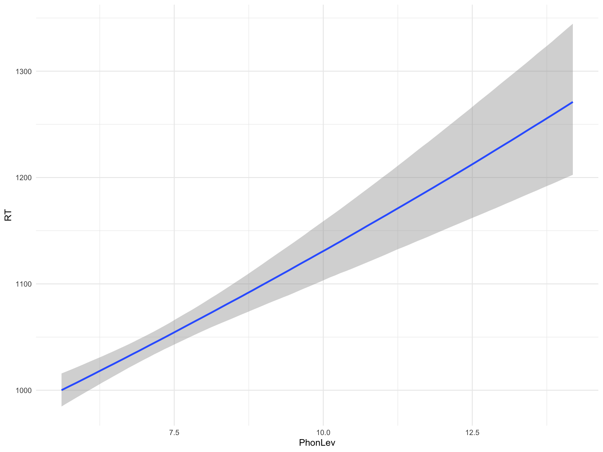
Figure 1: Predicted effect of mean phone-level distance on RTs from a Bayesian regression model.

Predicted RTs at representative values of `PhonLev`

brm_log_draws <- as_draws_df(brm_log)

brm_log_draws <- brm_log_draws |> 
  mutate(
    # RTs when PhonLev is 5
    rt_05 = exp(b_Intercept + b_PhonLev * 5),
    # RTs when PhonLev is 10
    rt_10 = exp(b_Intercept + b_PhonLev * 10),
    # RTs when PhonLev is 15
    rt_15 = exp(b_Intercept + b_PhonLev * 15),
  )

Calculating CrIs from the draws

library(posterior)

brm_log_cri <- brm_log_draws |> 
  select(rt_05, rt_10, rt_15) |> 
  pivot_longer(everything()) |> 
  group_by(name) |> 
  summarise(
    # Use quantile2() from posterior package
    lo_95 = round(quantile2(value, 0.025)),
    hi_95 = round(quantile2(value, 0.0975))
  )

brm_log_cri

# A tibble: 3 × 3
  name  lo_95 hi_95
  <chr> <dbl> <dbl>
1 rt_05   926   932
2 rt_10  1059  1068
3 rt_15  1174  1200

Summary

Quick and dirty diagnostics:

MCMC traces: hairy caterpillars, no divergent transitions.
\(\hat{R}\): should be 1 (> 1 means non-convergence).
Effective Sample Size (ESS): should be large enough.
Posterior Predictive Checks: predicted outcome distribution should match the empirical distribution.

brm() warns you about divergent transition, \(\hat{R} > 1\) and low ESS and how to fix them.
- This usually involves increasing the number of iterations and/or other MCMC tricks.
Posterior predictive checks are based on visual inspection only.