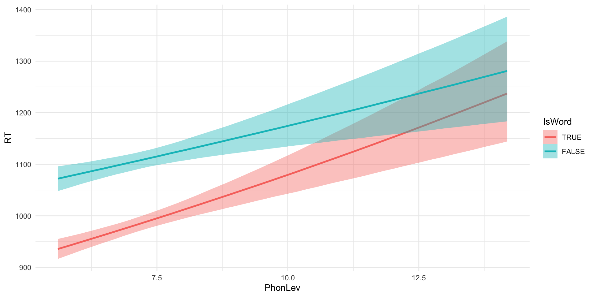
Introduction to Bayesian regression models

05 - Interactions

Stefano Coretta

University of Edinburgh

MALD

Figure 1: RTs by lexical status and mean phone-level distance.

MALD: IsWord and PhonLev

Research questions

  1. Does the lexical status of the word affect RTs?

  2. Does the mean phone-level distance affect RTs?

  3. Does the effect of mean phone-level distance differ depending on the lexical status?

For pedagogical reasons we fitted many regression models so far, but you should fit a single model to answer these questions.

Interactions

\[ \begin{align} RT_i & \sim Lognormal(\mu_i, \sigma_i)\\ log(\mu_i) & = \beta_1 \cdot W_{\text{T}[i]} + \beta_2 \cdot W_{\text{F}[i]}\\ & + \beta_3 \cdot PL_{W_\text{T}[i]} + \beta_4 \cdot PL_{W_\text{F}[i]}\\ \end{align} \]

We allow the model to estimate the PhonLev effect for real words and nonce words separately:

  • \(\beta_3\) is the effect of PhonLev when the word is real (\(PL_{W_\text{T}}\)).

  • \(\beta_4\) is the effect of PhonLev in nonce words (\(PL_{W_\text{F}}\)).

Regression with interaction

brm_int <- brm(
  RT ~ 0 + IsWord + IsWord:PhonLev,
  data = mald,
  family = lognormal,
  cores = 4,
  seed = 9812,
  file = "data/cache/brm_int.rds"
)

brm_int
 Family: lognormal 
  Links: mu = identity; sigma = identity 
Formula: RT ~ 0 + IsWord + IsWord:PhonLev 
   Data: mald (Number of observations: 3000) 
  Draws: 4 chains, each with iter = 2000; warmup = 1000; thin = 1;
         total post-warmup draws = 4000

Regression Coefficients:
                    Estimate Est.Error l-95% CI u-95% CI Rhat Bulk_ESS Tail_ESS
IsWordTRUE              6.62      0.04     6.54     6.70 1.00     1888     1924
IsWordFALSE             6.82      0.04     6.74     6.90 1.00     1414     1810
IsWordTRUE:PhonLev      0.03      0.01     0.02     0.04 1.00     1890     1877
IsWordFALSE:PhonLev     0.02      0.01     0.01     0.03 1.00     1438     1791

Further Distributional Parameters:
      Estimate Est.Error l-95% CI u-95% CI Rhat Bulk_ESS Tail_ESS
sigma     0.28      0.00     0.27     0.29 1.00     2673     2072

Draws were sampled using sampling(NUTS). For each parameter, Bulk_ESS
and Tail_ESS are effective sample size measures, and Rhat is the potential
scale reduction factor on split chains (at convergence, Rhat = 1).

RQ 3: Does the effect of mean phone-level distance differ depending on the lexical status?

brm_int_draws <- as_draws_df(brm_int) |> 
  mutate(
    # Back ticks `` are necessary because the column names have colons ":"
    
    phonlev_diff = `b_IsWordFALSE:PhonLev` - `b_IsWordTRUE:PhonLev`
  )

Difference in effect of PhonLev in nonce vs real words

brm_int_draws |> 
  ggplot(aes(phonlev_diff)) +
  stat_halfeye() +
  labs(
    x = "Difference (log)",
    y = element_blank()
  )

Difference in effect of PhonLev in nonce vs real words

Figure 2: Predicted difference in PhonLev effect in nonce vs real words.

CrIs of the difference in effect of PhonLev

library(posterior)

brm_int_draws |> 
  summarise(
    lo_95 = quantile2(phonlev_diff, 0.025), hi_95 = quantile2(phonlev_diff, 0.975),
    lo_90 = quantile2(phonlev_diff, 0.5), hi_90 = quantile2(phonlev_diff, 0.95),
    lo_80 = quantile2(phonlev_diff, 0.1), hi_80 = quantile2(phonlev_diff, 0.9),
    lo_70 = quantile2(phonlev_diff, 0.15), hi_70 = quantile2(phonlev_diff, 0.85)
  ) |> 

  # Some pivot magic to make it prettier
  pivot_longer(everything()) |> 
  separate(name, c("boundary", "interval")) |> 
  pivot_wider(names_from = boundary) |> 
  mutate(lo = round(lo, 4), hi = round(hi, 4))
# A tibble: 4 × 3
  interval      lo      hi
  <chr>      <dbl>   <dbl>
1 95       -0.0265  0.003 
2 90       -0.0118  0.0007
3 80       -0.0215 -0.0023
4 70       -0.0196 -0.0042

Plot the model predictions

conditional_effects(brm_int, "PhonLev:IsWord")

Quantify the lexical status difference (log)

phonlev_diff_5_10 <- brm_int_draws |> 
  mutate(
    true_5 = b_IsWordTRUE + `b_IsWordTRUE:PhonLev` * 5,
    false_5 = b_IsWordFALSE + `b_IsWordFALSE:PhonLev` * 5,
    true_10 = b_IsWordTRUE + `b_IsWordTRUE:PhonLev` * 10,
    false_10 = b_IsWordFALSE + `b_IsWordFALSE:PhonLev` * 10,
    ft_5 = false_5 - true_5,
    ft_10 = false_10 - true_10
  ) |> 
  select(ft_5, ft_10)

phonlev_diff_5_10
# A tibble: 4,000 × 2
    ft_5  ft_10
   <dbl>  <dbl>
 1 0.149 0.0606
 2 0.108 0.0901
 3 0.149 0.0913
 4 0.156 0.101 
 5 0.120 0.0950
 6 0.138 0.0918
 7 0.166 0.0445
 8 0.203 0.0337
 9 0.156 0.0435
10 0.164 0.0782
# ℹ 3,990 more rows

Plot the lexical status difference (log)

phonlev_diff_5_10 |> 
  pivot_longer(everything()) |> 
  ggplot(aes(value, name)) +
  stat_halfeye()

Figure 3

Quantify the lexical status difference (ms)

phonlev_diff_5_10_ms <- brm_int_draws |> 
  mutate(
    true_5 = exp(b_IsWordTRUE + `b_IsWordTRUE:PhonLev` * 5),
    false_5 = exp(b_IsWordFALSE + `b_IsWordFALSE:PhonLev` * 5),
    true_10 = exp(b_IsWordTRUE + `b_IsWordTRUE:PhonLev` * 10),
    false_10 = exp(b_IsWordFALSE + `b_IsWordFALSE:PhonLev` * 10),
    ft_5 = false_5 - true_5,
    ft_10 = false_10 - true_10
  ) |> 
  select(ft_5, ft_10)

phonlev_diff_5_10_ms
# A tibble: 4,000 × 2
    ft_5 ft_10
   <dbl> <dbl>
 1  142.  64.3
 2  102.  97.1
 3  142.  99.3
 4  149. 109. 
 5  113. 103. 
 6  129. 100. 
 7  158.  48.5
 8  192.  36.8
 9  148.  46.6
10  155.  86.5
# ℹ 3,990 more rows

Plot the lexical status difference (ms)

phonlev_diff_5_10_ms |> 
  pivot_longer(everything()) |> 
  ggplot(aes(value, name)) +
  stat_halfeye()

Figure 4

Summary

  • Bayesian statistics is a framework for doing inference (i.e. learning something about a population from a sample).

  • The Bayesian framework is based on estimating uncertainty with probability distributions on parameters.

  • Bayesian regressions are a flexible way to model data.

  • What you learned today can be transferred to other types of regression models (Bernoulli, cumulative, ordinal, categorical, beta, …).