Introduction to Bayesian regression models

02 - Bayesian regression

Stefano Coretta

University of Edinburgh

Regression models

• Simplest regression model:

\[ y \sim \beta_0 + \beta_1 \cdot x \]

• where \(y\) and \(x\) are numeric variables.

• https://stefanocoretta.shinyapps.io/lines/

MALD

Does the mean phone-level distance affect reaction times?

• Mean phone-level distance is a proxy of word “uniqueness”.

• More unique words should take longer to recognise as real words because there are less competitors (i.e. similar words) that can have a facilitatory effect on recognition.

MALD: RT and PhonLev

Figure 1: Scatter plot of mean phone-level distance vs reaction times.

MALD: regression

\[ RT \sim \beta_0 + \beta_1 \cdot \text{PhonLev} \]

or

\[ \begin{align} RT & \sim \beta_0 + \beta_1 \cdot \text{PhonLev} + \epsilon\\ \epsilon & \sim Gaussian(0, \sigma) \end{align} \]

or

\[ \begin{align} RT & \sim Gaussian(\mu, \sigma)\\ \mu & = \beta_0 + \beta_1 \cdot \text{PhonLev}\\ \end{align} \]

The model estimates the posterior probability distributions of \(\beta_0, \beta_1, \sigma\).

MALD: regression

brm_lev <- brm(
  RT ~ 1 + PhonLev,
  data = mald,
  family = "gaussian",
  file = "./data/cache/brm_lev.rds",
  chains = 4, 
  iter = 2000,
  cores = 4
)

summary(brm_lev)

 Family: gaussian 
  Links: mu = identity; sigma = identity 
Formula: RT ~ 1 + PhonLev 
   Data: mald (Number of observations: 3000) 
  Draws: 4 chains, each with iter = 2000; warmup = 1000; thin = 1;
         total post-warmup draws = 4000

Regression Coefficients:
          Estimate Est.Error l-95% CI u-95% CI Rhat Bulk_ESS Tail_ESS
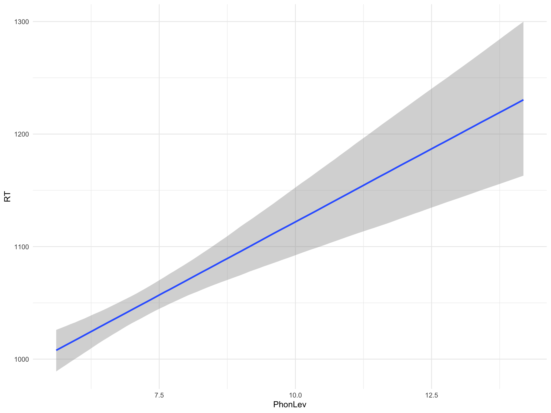
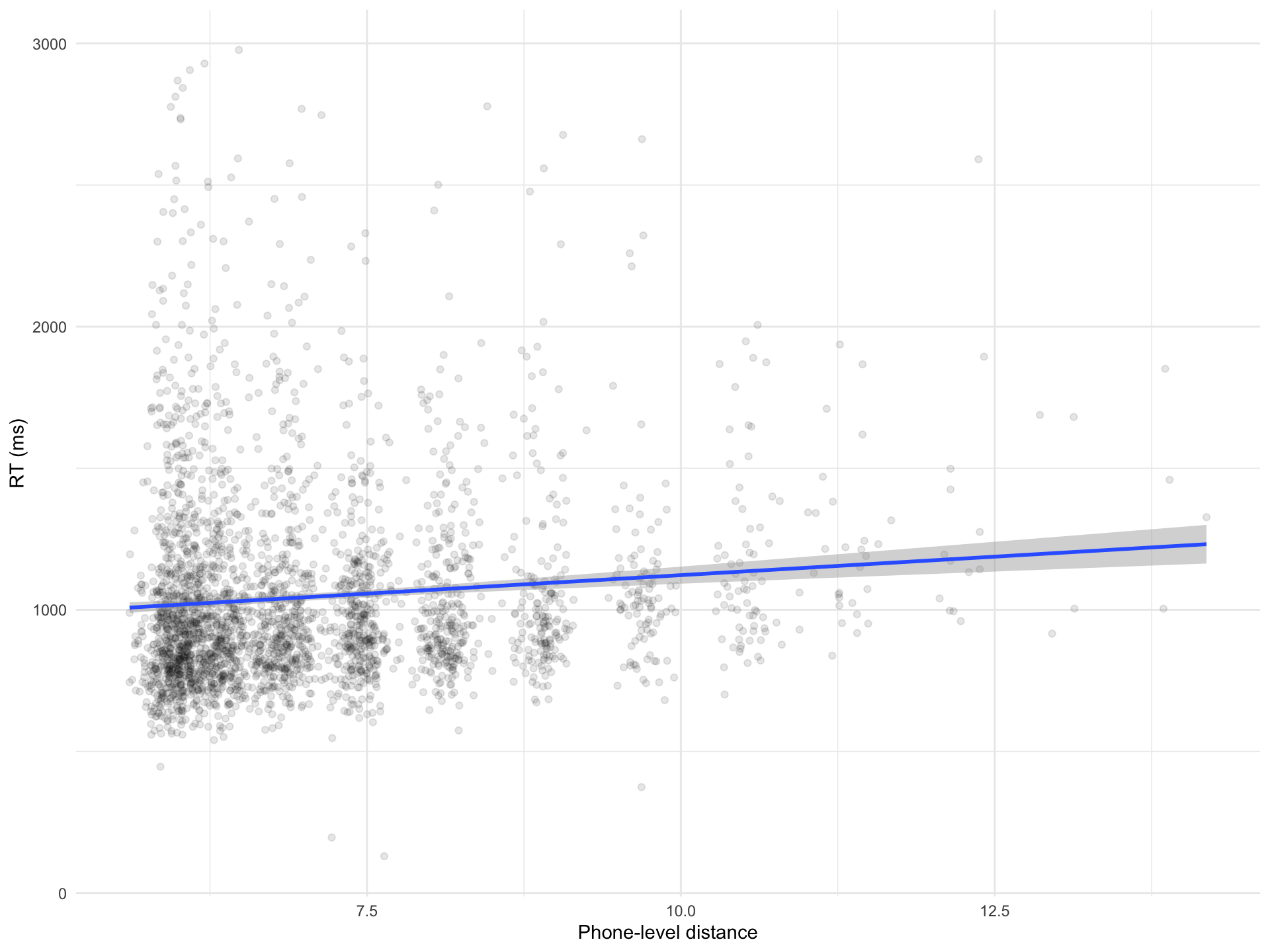
Intercept   861.62     35.11   793.25   929.05 1.00     4139     2815
PhonLev      26.05      4.85    16.70    35.40 1.00     4169     2866

Further Distributional Parameters:
      Estimate Est.Error l-95% CI u-95% CI Rhat Bulk_ESS Tail_ESS
sigma   345.95      4.54   337.09   354.71 1.00     3849     2919

Draws were sampled using sampling(NUTS). For each parameter, Bulk_ESS
and Tail_ESS are effective sample size measures, and Rhat is the potential
scale reduction factor on split chains (at convergence, Rhat = 1).

Interpret the summary: Intercept

Regression Coefficients:
          Estimate Est.Error l-95% CI u-95% CI Rhat Bulk_ESS Tail_ESS
Intercept   861.62     35.11   793.25   929.05 1.00     4139     2815
PhonLev      26.05      4.85    16.70    35.40 1.00     4169     2866

Intercept is \(\beta_0\).

• \(\beta_0\) is the expected mean RT when PhonLev is 0.

• The posterior probability distribution of \(\beta_0\) is \(\mathcal{P}(862, 35)\).

• There is a 95% probability that the mean RTs when PhonLev is 0 is between 793 and 929 ms, conditional on the model and data. This is the 95% Credible Interval (CrI) of \(\mathcal{P}(862, 35)\).

Interpret the summary: PhonLev

Regression Coefficients:
          Estimate Est.Error l-95% CI u-95% CI Rhat Bulk_ESS Tail_ESS
Intercept   861.62     35.11   793.25   929.05 1.00     4139     2815
PhonLev      26.05      4.85    16.70    35.40 1.00     4169     2866

PhonLev is \(\beta_1\).

• \(\beta_1\) is the expected difference in RT for each unit change of PhonLev.

• The posterior probability distribution of \(\beta_1\) is \(\mathcal{P}(26, 5)\).

• There is a 95% probability that each unit change of PhonLev corresponds to a change in mean RT between +17 and +35 ms, conditional on the model and data. This is the 95% Credible Interval (CrI) of \(\mathcal{P}(26, 5)\).

Effect of PhonLev on RTs

conditional_effects(brm_lev, "PhonLev")

Figure 2: Predicted effect of mean phone-level distance on RTs from a Bayesian regression model.

MCMC draws

brm_lev_draws <- as_draws_df(brm_lev)

brm_lev_draws

# A draws_df: 1000 iterations, 4 chains, and 6 variables
   b_Intercept b_PhonLev sigma Intercept lprior   lp__
1          878        25   344      1054    -13 -21803
2          880        25   345      1056    -13 -21803
3          872        25   340      1050    -13 -21803
4          821        32   341      1047    -13 -21803
5          838        30   344      1054    -13 -21803
6          859        25   352      1037    -13 -21803
7          861        25   350      1039    -13 -21803
8          861        28   348      1057    -13 -21803
9          916        20   346      1056    -13 -21804
10         844        29   350      1052    -13 -21803
# ... with 3990 more draws
# ... hidden reserved variables {'.chain', '.iteration', '.draw'}

Predicted RTs at representative values of PhonLev

range(mald$PhonLev)

[1]  5.608767 14.186571

brm_lev_draws <- brm_lev_draws |> 
  mutate(
    # RTs when PhonLev is 5
    rt_05 = b_Intercept + b_PhonLev * 5,
    # RTs when PhonLev is 10
    rt_10 = b_Intercept + b_PhonLev * 10,
    # RTs when PhonLev is 15
    rt_15 = b_Intercept + b_PhonLev * 15,
  )

brm_lev_draws |> 
  select(rt_05, rt_10, rt_15)

# A tibble: 4,000 × 3
   rt_05 rt_10 rt_15
   <dbl> <dbl> <dbl>
 1 1002. 1127. 1251.
 2 1004. 1128. 1252.
 3  998. 1123. 1249.
 4  980. 1140. 1299.
 5  990. 1142. 1293.
 6  985. 1111. 1236.
 7  987. 1112. 1238.
 8  999. 1138. 1276.
 9 1015. 1113. 1211.
10  990. 1137. 1284.
# ℹ 3,990 more rows

Predicted RTs at representative values of PhonLev: plot

library(ggdist)

brm_lev_draws |> 
  select(rt_05, rt_10, rt_15) |> 
  
  # Pivot so to make plotting easier
  pivot_longer(everything()) |> 
  # Pivot creates a name column with values `rt_05, rt_10, rt_15`
  # and a value column with the draws values
  
  ggplot(aes(value, name)) +
  # Stat halfeye from ggdist
  stat_halfeye() +
  labs(
    caption = "Point = median, thick line = 66% CrI, thin line = 95% CrI."
  )

Predicted RTs at representative values of PhonLev: plot

Figure 3: Predicted RTs at representative values of mean phon-level distance.

Calculating CrIs from the draws

library(posterior)

brm_lev_cri <- brm_lev_draws |> 
  select(rt_05, rt_10, rt_15) |> 
  pivot_longer(everything()) |> 
  group_by(name) |> 
  summarise(
    # Use quantile2() from posterior package
    lo_95 = round(quantile2(value, 0.025)),
    hi_95 = round(quantile2(value, 0.0975))
  )

brm_lev_cri

# A tibble: 3 × 3
  name  lo_95 hi_95
  <chr> <dbl> <dbl>
1 rt_05   968   976
2 rt_10  1092  1103
3 rt_15  1177  1203

Width of the CrIs

brm_lev_cri |> 
  mutate(
    cri_width = hi_95 - lo_95
  )

# A tibble: 3 × 4
  name  lo_95 hi_95 cri_width
  <chr> <dbl> <dbl>     <dbl>
1 rt_05   968   976         8
2 rt_10  1092  1103        11
3 rt_15  1177  1203        26

Reporting

We fitted a Bayesian Gaussian regression model with brms (Bürkner 2017) in R 4.5.0 (R Core Team 2025). The model had reaction times as the outcome variable and mean phone-level distance as the only predictor. The model was fitted with 4 MCMC chains and 2000 iterations per chains. The default brms priors were used.

According to the model results, for every increase of mean phone-level distance by 1 unit, reaction times increase by 17-35 ms, at 95% probability (\(\beta\) = 26.05, SD = 4.85). The 95% CrIs of the predicted reaction times at representative values of mean distance are: 968-976 ms for mean distance = 5, 1092-1103 ms for mean distance = 10, 1177-1203 for mean distance = 15.

References

Bürkner, Paul-Christian. 2017. “Brms: An r Package for Bayesian Multilevel Models Using Stan.” Journal of Statistical Software 80 (1): 128. https://doi.org/10.18637/jss.v080.i01.

R Core Team. 2025. R: A Language and Environment for Statistical Computing. Vienna, Austria: R Foundation for Statistical Computing. https://www.R-project.org/.