Introduction to Bayesian regression models

01 - Basics

Stefano Coretta

University of Edinburgh

Download the workshop materials

• Download the workshop repository from: https://github.com/stefanocoretta/learnBayes.

Schedule

Times	Topic
9.00-10.30	Introduction to Bayesian modelling
10.30-11.00	Break
11.00-12.30	Bayesian regression + Diagnostics
12.30-14.30	Lunch break
14.30-16.00	Categorical predictors + Interactions
16.00-16.30	Break
16.30-18.00	Bayesian modelling Q&A

One model to rule them all.
One model to find them.
One model to bring them all
And in the darkness bind them.

(No, I couldn’t translate ‘model’ into Black Speech, alas…)

Now enter The Regression Model

Now enter The Bayesian Regression Model

All about the Bayes

Within the NHST (Frequentist) framework, the main analysis output is:

• Point estimates of predictors’ parameters (with standard error).
• p-values.

See Gigerenzer (2004), Gigerenzer, Krauss, and Vitouch (2004), Gigerenzer (2018) for problems with the “Null Ritual”.

Within the Bayesian framework, the main analysis output is:

• Probability distributions of predictors’ parameters.

An example: MALD

Massive Auditory Lexical Decision (MALD) data (Tucker et al. 2019):

• Auditory Lexical Decision task with real and nonce English words.
• Reaction times and accuracy.
• Total 521 subjects; subset of 30 subjects, 100 observations each.

MALD data

mald

# A tibble: 3,000 × 7
   Subject Item         IsWord PhonLev    RT ACC       RT_log
   <chr>   <chr>        <fct>    <dbl> <int> <fct>      <dbl>
 1 15345   nihnaxr      FALSE     5.84   945 correct     6.85
 2 15345   skaep        FALSE     6.03  1046 incorrect   6.95
 3 15345   grandparents TRUE     10.3    797 correct     6.68
 4 15345   sehs         FALSE     5.88  2134 correct     7.67
 5 15345   cousin       TRUE      5.78   597 correct     6.39
 6 15345   blowup       TRUE      6.03   716 correct     6.57
 7 15345   hhehrnzmaxn  FALSE     7.30  1985 correct     7.59
 8 15345   mantic       TRUE      6.21  1591 correct     7.37
 9 15345   notable      TRUE      6.82   620 correct     6.43
10 15345   prowthihviht FALSE     7.68  1205 correct     7.09
# ℹ 2,990 more rows

MALD: phone-level distance and lexical status

Let’s investigate the effects of the following on Reaction Times (RTs):

• PhonLev: mean phone-level Levenshtein distance of the item from all other entries.
  • An alternative to neighbourhood density.
• IsWord: lexical status (real word vs nonce word).

MALD: phone-level distance and lexical status

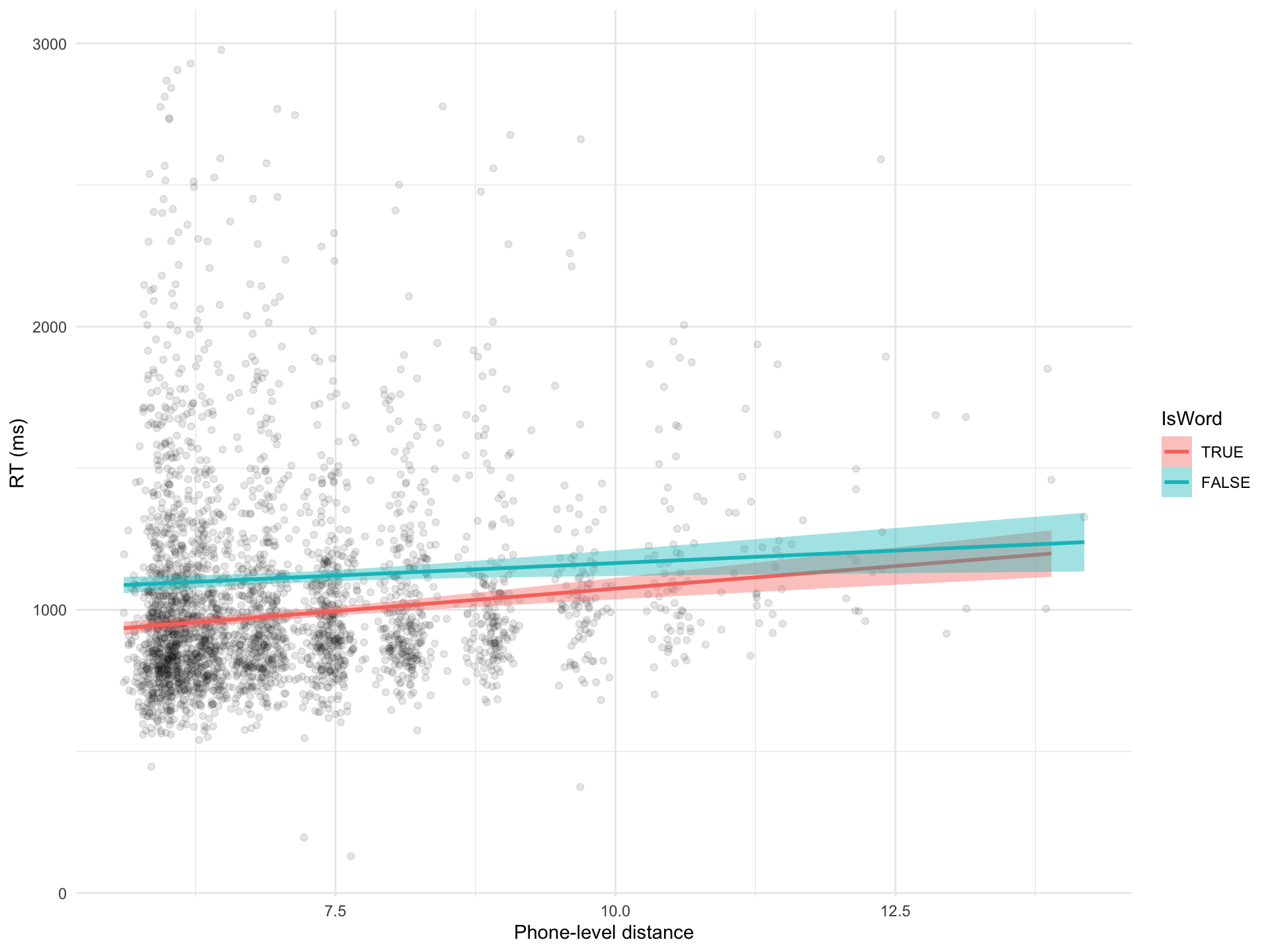
Figure 1: Scatter plot of mean phone-level distance vs reaction times.

A frequentist regression model

lm_1 <- lmer(
  RT ~
    PhonLev +
    IsWord +
    PhonLev:IsWord +
    (1 | Subject),
  data = mald
)

A frequentist regression model: summary

summary(lm_1)

Linear mixed model fit by REML. t-tests use Satterthwaite's method [
lmerModLmerTest]
Formula: RT ~ PhonLev + IsWord + PhonLev:IsWord + (1 | Subject)
   Data: mald

REML criterion at convergence: 43232.4

Scaled residuals: 
    Min      1Q  Median      3Q     Max 
-3.5511 -0.5985 -0.2439  0.3185  5.6906 

Random effects:
 Groups   Name        Variance Std.Dev.
 Subject  (Intercept)  11032   105.0   
 Residual             104648   323.5   
Number of obs: 3000, groups:  Subject, 30

Fixed effects:
                    Estimate Std. Error       df t value Pr(>|t|)    
(Intercept)          754.965     49.687  862.751  15.195  < 2e-16 ***
PhonLev               32.148      6.389 2970.933   5.032 5.15e-07 ***
IsWordFALSE          212.440     65.453 2972.588   3.246  0.00118 ** 
PhonLev:IsWordFALSE  -11.620      9.076 2972.817  -1.280  0.20055    
---
Signif. codes:  0 '***' 0.001 '**' 0.01 '*' 0.05 '.' 0.1 ' ' 1

Correlation of Fixed Effects:
            (Intr) PhonLv IWFALS
PhonLev     -0.907              
IsWordFALSE -0.647  0.690       
PhL:IWFALSE  0.640 -0.705 -0.983

A frequentist regression model: plot predictions

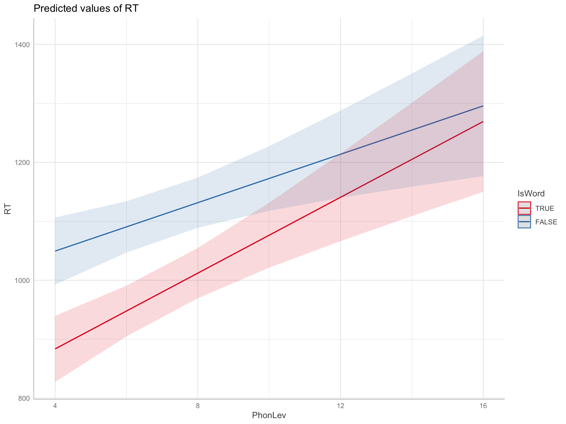
Figure 2: Predicted Reaction Times based on a frequentist regression model.

Increase model complexity

lm_2 <- lmer(
  RT ~
    PhonLev +
    IsWord +
    PhonLev:IsWord +
    (PhonLev*IsWord | Subject),
  data = mald
)

boundary (singular) fit: see help('isSingular')

Warning: Model failed to converge with 1 negative eigenvalue: -2.5e+01

Let’s go Bayesian!

A Bayesian regression model

library(brms)

brm_1 <- brm(
  RT ~
    PhonLev +
    IsWord +
    PhonLev:IsWord +
    (PhonLev * IsWord | Subject),
  data = mald,
  family = gaussian()
)

A Bayesian regression model: summary

brm_1

 Family: gaussian 
  Links: mu = identity; sigma = identity 
Formula: RT ~ PhonLev + IsWord + PhonLev:IsWord + (PhonLev * IsWord | Subject) 
   Data: mald (Number of observations: 3000) 
  Draws: 4 chains, each with iter = 4000; warmup = 2000; thin = 1;
         total post-warmup draws = 8000

Multilevel Hyperparameters:
~Subject (Number of levels: 30) 
                                     Estimate Est.Error l-95% CI u-95% CI Rhat
sd(Intercept)                           89.60     32.39    23.91   163.00 1.00
sd(PhonLev)                              6.81      4.93     0.32    17.93 1.00
sd(IsWordFALSE)                        112.59     40.17    51.48   214.51 1.00
sd(PhonLev:IsWordFALSE)                  6.49      5.27     0.22    19.83 1.00
cor(Intercept,PhonLev)                  -0.31      0.44    -0.90     0.67 1.00
cor(Intercept,IsWordFALSE)               0.43      0.29    -0.22     0.89 1.00
cor(PhonLev,IsWordFALSE)                -0.19      0.44    -0.87     0.74 1.00
cor(Intercept,PhonLev:IsWordFALSE)      -0.02      0.45    -0.82     0.82 1.00
cor(PhonLev,PhonLev:IsWordFALSE)        -0.08      0.45    -0.84     0.78 1.00
cor(IsWordFALSE,PhonLev:IsWordFALSE)    -0.30      0.47    -0.95     0.70 1.00
                                     Bulk_ESS Tail_ESS
sd(Intercept)                             928      371
sd(PhonLev)                               750     1760
sd(IsWordFALSE)                          1190      806
sd(PhonLev:IsWordFALSE)                  1175      862
cor(Intercept,PhonLev)                   2348     3006
cor(Intercept,IsWordFALSE)               1012      661
cor(PhonLev,IsWordFALSE)                  811     1085
cor(Intercept,PhonLev:IsWordFALSE)       5085     3160
cor(PhonLev,PhonLev:IsWordFALSE)         3771     3295
cor(IsWordFALSE,PhonLev:IsWordFALSE)     1816     1348

Regression Coefficients:
                    Estimate Est.Error l-95% CI u-95% CI Rhat Bulk_ESS Tail_ESS
Intercept             755.02     48.28   659.98   848.85 1.00     3920     5309
PhonLev                31.99      6.52    18.99    44.79 1.00     4604     5222
IsWordFALSE           208.23     67.99    75.34   341.44 1.00     3642     4658
PhonLev:IsWordFALSE   -11.06      9.12   -28.68     6.71 1.00     3743     4748

Further Distributional Parameters:
      Estimate Est.Error l-95% CI u-95% CI Rhat Bulk_ESS Tail_ESS
sigma   320.31      4.16   312.30   328.40 1.00     7998     5470

Draws were sampled using sampling(NUTS). For each parameter, Bulk_ESS
and Tail_ESS are effective sample size measures, and Rhat is the potential
scale reduction factor on split chains (at convergence, Rhat = 1).

A Bayesian regression model: plot predictions

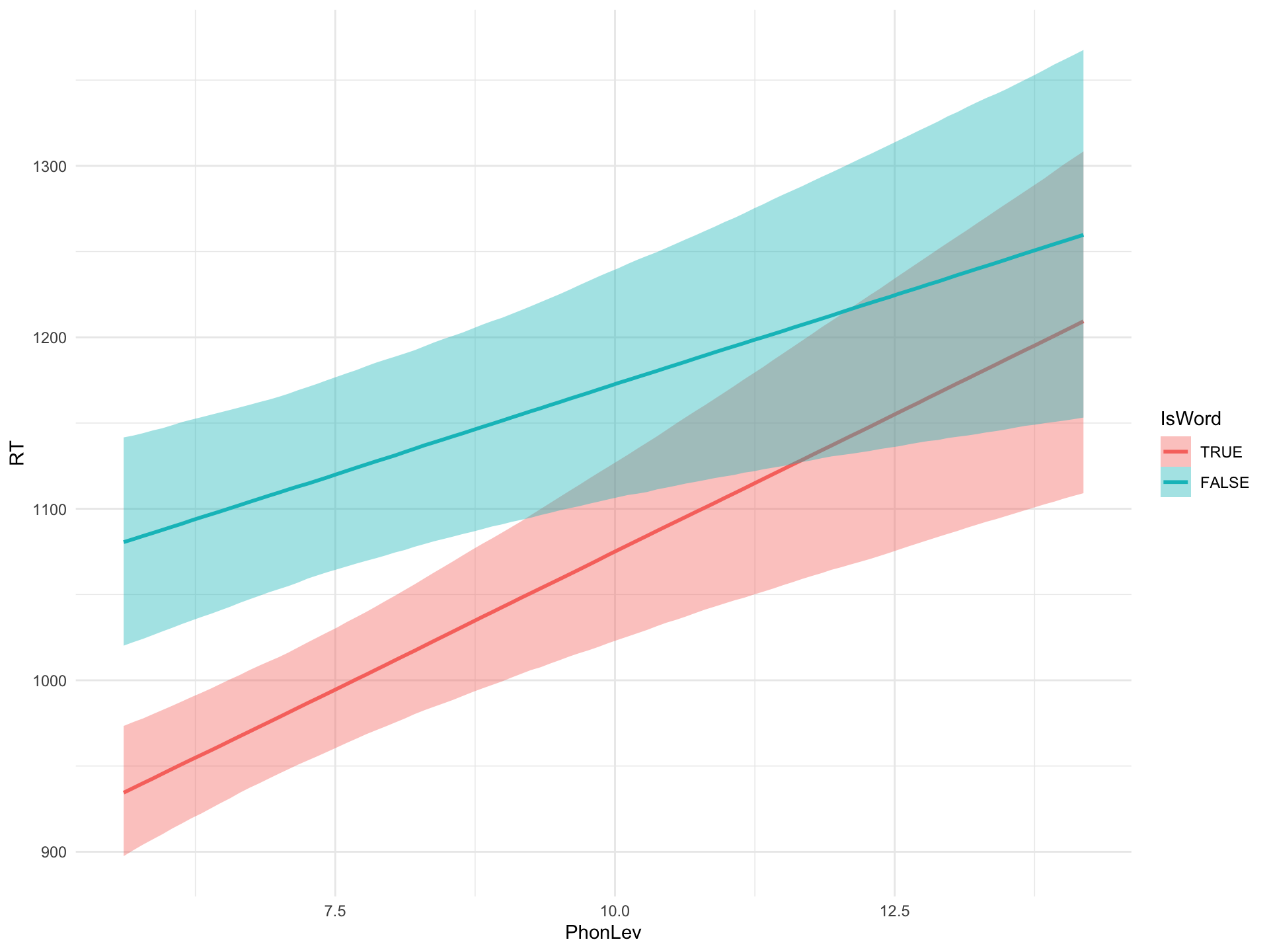
Figure 3: Predicted RTs based on a Bayesian regression model.

Let’s start small: A Gaussian model

\[ RT \sim Gaussian(\mu, \sigma) \]

• Reaction Times \(RT\)

• distributed according to \(\sim\)

• a Gaussian distribution \(Gaussian()\)

• with mean \(\mu\) and standard deviation \(\sigma\).

We start with a Gaussian model for pedagogical reasons. You would usually start with the model you need to answer your research questions.

Uncertainty of parameters

\[ \begin{align} RT & \sim Gaussian(\mu, \sigma)\\ \mu & \sim \mathcal{P}(\mu_1, \sigma_1)\\ \sigma & \sim \mathcal{P}(\mu_2, \sigma_2) \end{align} \]

• Uncertainty can be expressed with probability distributions. We use \(\mathcal{P}\) as a generic (undetermined) probability distribution.

• The Gaussian model estimates the probability distributions \(\mathcal{P}\) of \(\mu\) and \(\sigma\) from the data.

• These probability distributions \(\mathcal{P}\) are called posterior probability distributions.

• They can be summarised with \(\mu_1, \sigma_1, \mu_2, \sigma_2\).

Gaussian model of RTs

Try it yourself!

brm_2 <- brm(
  # formula = 
  RT ~ 1,
  data = mald,
  # Specify the distribution family of the outcome
  family = gaussian()
)

• The model estimates the probability distributions of \(\mu\) and \(\sigma\).

• To do so, a sampling algorithm is used (Markov Chain Monte Carlo, MCMC).

MCMC what?

Markov Chain Monte Carlo

• MCMC simulation: https://chi-feng.github.io/mcmc-demo/app.html

• More on MCMC

  • https://elizabethpankratz.github.io/bayes_stat/day1/mcmc.html

  • http://elevanth.org/blog/2017/11/28/build-a-better-markov-chain/

Technicalities

brm_2 <- brm(
  RT ~ 1,
  data = mald,
  family = gaussian(),
  
  # TECHNICAL STUFF
  # Save model output to file
  file = "./data/cache/brm_2.rds",
  # Number of MCMC chains
  chains = 4, 
  # Number of iterations per chain
  iter = 2000,
  # Number of cores to use (one per chain)
  cores = 4
)

You can find out how many cores your laptop has with parallel::detectCores().

The model summary

brm_2

 Family: gaussian 
  Links: mu = identity; sigma = identity 
Formula: RT ~ 1 
   Data: mald (Number of observations: 3000) 
  Draws: 4 chains, each with iter = 2000; warmup = 1000; thin = 1;
         total post-warmup draws = 4000

Regression Coefficients:
          Estimate Est.Error l-95% CI u-95% CI Rhat Bulk_ESS Tail_ESS
Intercept  1046.57      6.38  1034.21  1058.95 1.00     3165     2707

Further Distributional Parameters:
      Estimate Est.Error l-95% CI u-95% CI Rhat Bulk_ESS Tail_ESS
sigma   347.57      4.52   338.77   356.50 1.00     3804     2833

Draws were sampled using sampling(NUTS). For each parameter, Bulk_ESS
and Tail_ESS are effective sample size measures, and Rhat is the potential
scale reduction factor on split chains (at convergence, Rhat = 1).

Interpret the summary: \(\mu\)

Regression Coefficients:
          Estimate Est.Error l-95% CI u-95% CI Rhat Bulk_ESS Tail_ESS
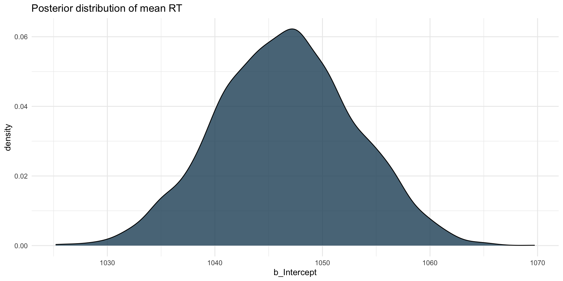
Intercept  1046.57      6.38  1034.21  1058.95 1.00     3165     2707

Intercept is \(\mu\).

\[ \begin{align} RT & \sim Gaussian(\mu, \sigma)\\ \mu & \sim \mathcal{P}(1046.57, 6.38)\\ \end{align} \]

• The posterior probability distribution of \(\mu\), i.e. of the mean RTs, is \(\mathcal{P}(1047, 6)\).

• There is a 95% probability that the mean RTs is between 1034 and 1059 ms, conditional on the model and data. This is the 95% Credible Interval (CrI) of \(\mathcal{P}(1047, 6)\).

Interpret the summary: \(\sigma\)

Further Distributional Parameters:
      Estimate Est.Error l-95% CI u-95% CI Rhat Bulk_ESS Tail_ESS
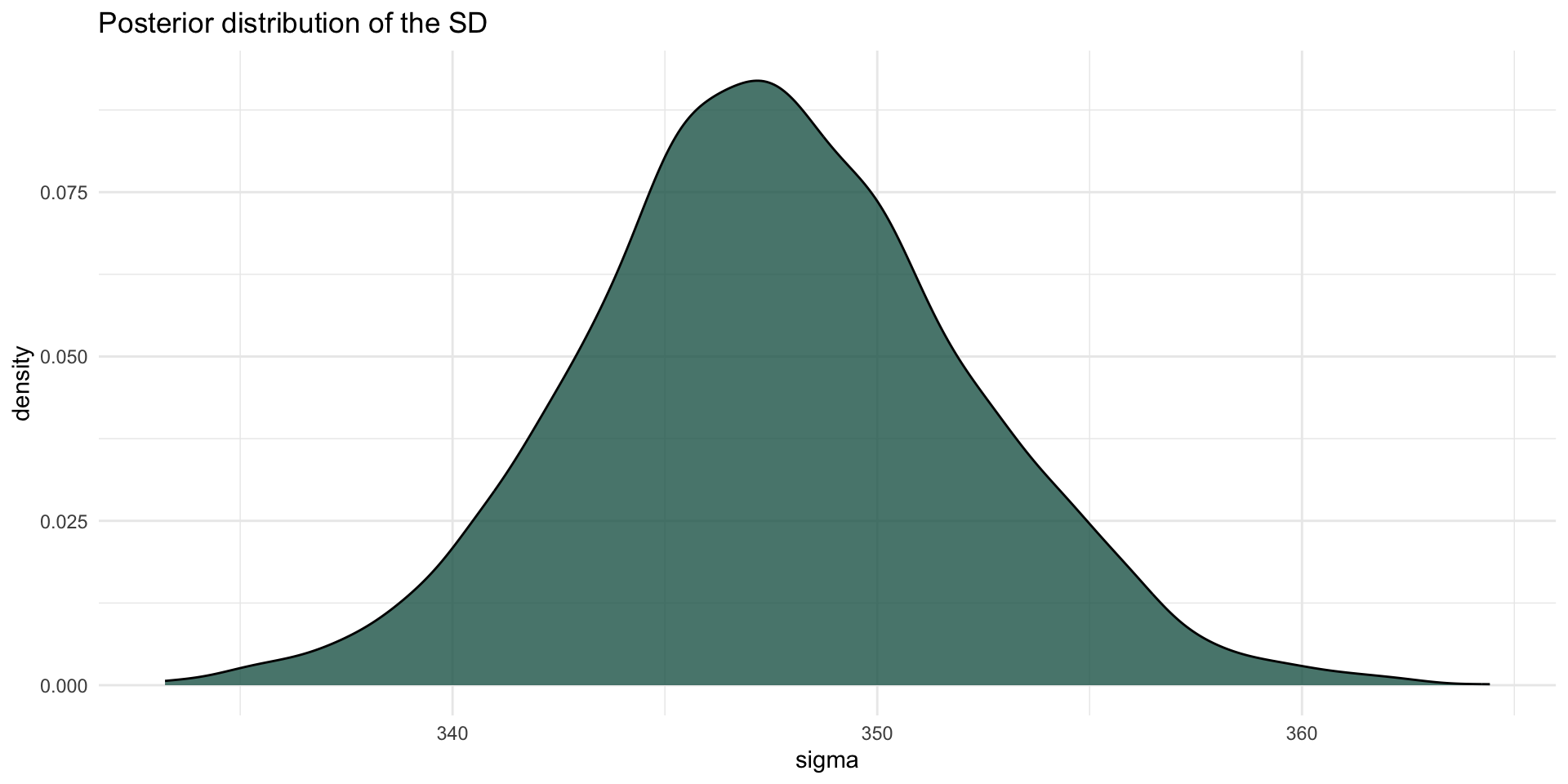
sigma   347.57      4.52   338.77   356.50 1.00     3804     2833

sigma is \(\sigma\).

\[ \begin{align} RT & \sim Gaussian(\mu, \sigma)\\ \mu & \sim \mathcal{P}(1046.57, 6.38)\\ \sigma & \sim \mathcal{P}(347.57, 4.52) \end{align} \]

• The posterior probability distribution of \(\sigma\), i.e. of the standard deviation of RTs, is \(\mathcal{P}(348, 5)\).

• There is a 95% probability that the RT standard deviation is between 339 and 357 ms, conditional on the model and data.

Posterior probabilities

• These are posterior probability distributions.
• They are always conditional on model and data.
• The summary reports 95% Credible Intervals (CrIs), but there is nothing special about 95% and you should obtain a set of intervals.

Model plot

plot(brm_2, combo = c("dens", "trace"))

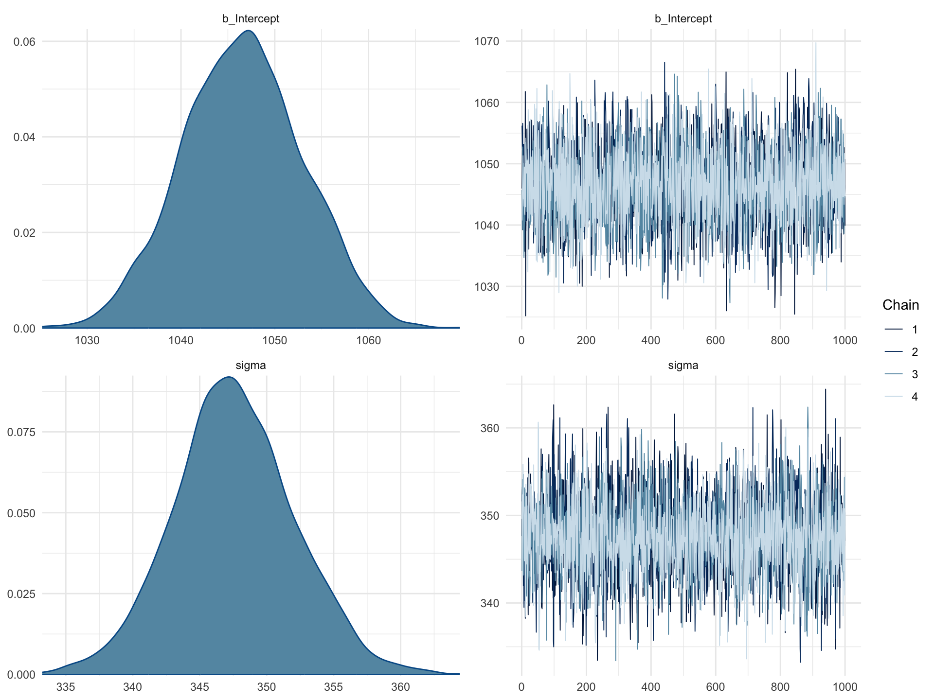
Figure 4: Density and trace plot of the Bayesian Gaussian model brm_2.

Extract the MCMC draws

brm_2_draws <- as_draws_df(brm_2)
brm_2_draws

# A draws_df: 1000 iterations, 4 chains, and 5 variables
   b_Intercept sigma Intercept lprior   lp__
1         1046   348      1046    -13 -21816
2         1052   353      1052    -13 -21817
3         1039   349      1039    -13 -21817
4         1045   343      1045    -13 -21817
5         1046   344      1046    -13 -21817
6         1050   348      1050    -13 -21816
7         1050   348      1050    -13 -21816
8         1044   345      1044    -13 -21816
9         1048   350      1048    -13 -21816
10        1036   345      1036    -13 -21818
# ... with 3990 more draws
# ... hidden reserved variables {'.chain', '.iteration', '.draw'}

Get parameters

To list all the names of the parameters in a model, use:

variables(brm_2)

[1] "b_Intercept" "sigma"       "Intercept"   "lprior"      "lp__"       

Posterior distribution: mean RT

Now you can plot the probability density of the draws using ggplot2.

brm_2_draws |>
  ggplot(aes(b_Intercept)) +
  geom_density(fill = "#214d65", alpha = 0.8) +
  labs(title = "Posterior distribution of mean RT")

Posterior distribution: mean RT

Posterior distribution: sigma

brm_2_draws |>
  ggplot(aes(sigma)) +
  geom_density(fill = "#1F6357", alpha = 0.8) +
  labs(title = "Posterior distribution of the SD")

Posterior distribution: sigma

Summary

• Bayesian statistics is a framework for doing inference (i.e. learning something about a population from a sample).

• The Bayesian framework is based on estimating uncertainty with probability distributions on parameters.

• The syntax you know from [g]lm[er]() works with brm() from the brms package.

• Results allow you to make statements like “There is a 95% probability that the difference between A and B is between q and w”.

References

Gigerenzer, Gerd. 2004. “Mindless Statistics.” The Journal of Socio-Economics 33 (5): 587606. https://doi.org/10.1016/j.socec.2004.09.033.

———. 2018. “Statistical Rituals: The Replication Delusion and How We Got There.” Advances in Methods and Practices in Psychological Science 1 (2): 198218. https://doi.org/10.1177/2515245918771329.

Gigerenzer, Gerd, Stefan Krauss, and Oliver Vitouch. 2004. “The Null Ritual. What You Always Wanted to Know about Significance Testing but Were Afraid to Ask.” In, 391408.

Tucker, Benjamin V, Daniel Brenner, Kyle Danielson D, Matthew C Kelley, Filip Nenadić, and Michelle Sims. 2019. “The Massive Auditory Lexical Decision (MALD) Database.” Behavior Research Methods 51 (3): 11871204. https://doi.org/10.3758/s13428-018-1056-1.