Using generalised additive models (GAM) with polar coordinates for assessing tongue contours

Read data

The package rticulate comes with a dataset containing spline data from two speakers of Italian.

library(rticulate)
data(tongue)
tongue
#> # A tibble: 3,612 × 28
#>    speaker seconds rec_date prompt label TT_di…¹ TT_ve…² TT_ab…³ TD_di…⁴ TD_ve…⁵
#>    <fct>     <dbl> <fct>    <fct>  <fct>   <dbl>   <dbl>   <dbl>   <dbl>   <dbl>
#>  1 it01       1.31 29/11/2… Dico … max_…    67.1   36.6    37.5     81.8   -4.95
#>  2 it01       1.20 29/11/2… Dico … max_…    77.9   -7.73    5.10    67.3  -34.3 
#>  3 it01       1.08 29/11/2… Dico … max_…    65.9   21.1    20.9     81.8   -4.07
#>  4 it01       1.12 29/11/2… Dico … max_…    64.4    8.76    6.46    81.5   -2.55
#>  5 it01       1.42 29/11/2… Dico … max_…    76.9   -4.72    2.55    75.8  -58.0 
#>  6 it01       1.35 29/11/2… Dico … max_…    78.1   -5.68    3.60    73.2   20.5 
#>  7 it01       1.07 29/11/2… Dico … max_…    69.9  -40.0    40.0     82.4   -5.12
#>  8 it01       1.17 29/11/2… Dico … max_…    78.0   -7.31    4.37    69.3   -3.37
#>  9 it01       1.28 29/11/2… Dico … max_…    67.1   34.5    33.4     81.4   -5.28
#> 10 it01       1.10 29/11/2… Dico … max_…    75.9  -23.5    22.0     81.0   -2.89
#> # … with 3,602 more rows, 18 more variables: TD_abs_velocity <dbl>,
#> #   TR_displacement <dbl>, TR_velocity <dbl>, TR_abs_velocity <dbl>,
#> #   fan_line <int>, X <dbl>, Y <dbl>, word <fct>, item <dbl>, ipa <fct>,
#> #   c1 <fct>, c1_phonation <fct>, vowel <fct>, anteropost <fct>, height <fct>,
#> #   c2 <fct>, c2_phonation <fct>, c2_place <fct>, and abbreviated variable
#> #   names ¹TT_displacement, ²TT_velocity, ³TT_abs_velocity, ⁴TD_displacement,
#> #   ⁵TD_velocity

Fit a polar GAM

The spline data is in cartesian coordinates. The function polar_gam() converts the coordinates to polar and fits a GAM to the data. Note that, unless you have a working method to normalise between speakers, it is recommended to fit separate models for each speaker.

The polar coordinates are calculated based on the origin of the probe, which is estimated if origin = NULL using the fan lines specified with the argument fan_lines (the defaults are c(10, 25)).

If you get an error relating to lm.fit, try to change the fan_lines to values different from the default.

tongue_it05 <- filter(tongue, speaker == "it05", vowel == "a", fan_line < 38) %>% droplevels()

polar_place <- polar_gam(
  Y ~
    s(X, by = c2_place),
  data = tongue_it05
)
#> The origin is x = 11.028937677505, y = -53.2813982686628.
summary(polar_place)
#> 
#> Family: gaussian 
#> Link function: identity 
#> 
#> Formula:
#> Y ~ s(X, by = c2_place)
#> 
#> Parametric coefficients:
#>             Estimate Std. Error t value Pr(>|t|)    
#> (Intercept) 62.75772    0.08464   741.5   <2e-16 ***
#> ---
#> Signif. codes:  0 '***' 0.001 '**' 0.01 '*' 0.05 '.' 0.1 ' ' 1
#> 
#> Approximate significance of smooth terms:
#>                        edf Ref.df     F p-value    
#> s(X):c2_placecoronal 4.576  5.614 142.7  <2e-16 ***
#> s(X):c2_placevelar   7.993  8.732 372.2  <2e-16 ***
#> ---
#> Signif. codes:  0 '***' 0.001 '**' 0.01 '*' 0.05 '.' 0.1 ' ' 1
#> 
#> R-sq.(adj) =  0.934   Deviance explained = 93.6%
#> fREML = 534.93  Scale est. = 2.0697    n = 289

The output model is in polar coordinates but it contains the origin coordinates so that plotting can be done in cartesian coordinates.

We can now plot the results from the model with plot_polar_smooths().

plot_polar_smooths(
  polar_place,
  X,
  c2_place
) +
  theme(legend.position = "top")

Multiple predictors

It is possible to specify multiple predictors in the model and then facet the plots.

tongue_it05 <- filter(tongue, speaker == "it05", fan_line < 38) %>% droplevels()

polar_multi <- polar_gam(
  Y ~
    s(X, by = c2_place) +
    s(X, by = vowel),
  data = tongue_it05
)
#> The origin is x = 11.0276270964655, y = -53.2776157001125.
summary(polar_multi)
#> 
#> Family: gaussian 
#> Link function: identity 
#> 
#> Formula:
#> Y ~ s(X, by = c2_place) + s(X, by = vowel)
#> 
#> Parametric coefficients:
#>             Estimate Std. Error t value Pr(>|t|)    
#> (Intercept)  61.9700     0.0768   806.9   <2e-16 ***
#> ---
#> Signif. codes:  0 '***' 0.001 '**' 0.01 '*' 0.05 '.' 0.1 ' ' 1
#> 
#> Approximate significance of smooth terms:
#>                        edf Ref.df      F  p-value    
#> s(X):c2_placecoronal 5.583  6.597  3.827 0.000724 ***
#> s(X):c2_placevelar   6.925  7.784  8.564  < 2e-16 ***
#> s(X):vowela          3.825  4.746  2.219 0.042102 *  
#> s(X):vowelo          2.573  3.003  2.176 0.086926 .  
#> s(X):vowelu          6.835  7.774 10.861  < 2e-16 ***
#> ---
#> Signif. codes:  0 '***' 0.001 '**' 0.01 '*' 0.05 '.' 0.1 ' ' 1
#> 
#> Rank: 45/46
#> R-sq.(adj) =  0.915   Deviance explained = 91.8%
#> fREML = 1986.9  Scale est. = 5.1237    n = 872

Th argument facet_terms can be used to specify the terms for the facets. If you desire to facet by more then one term, just add multiple terms separated by + (for example, facet_terms = vowel + voicing; only terms that have been included in the model can be used for faceting, for more examples see the vignettes of the tidymv package).

plot_polar_smooths(
  polar_multi,
  X,
  c2_place,
  facet_terms = vowel
) +
  theme(legend.position = "top")

Extract all predicted values

If your model includes other smooths, or you want to have more control over the plotting, you can use the function predict_polar_gam(). This function is based on tidymv::predict_gam(), and I suggest the reader to familiarise themselves with vignette("predict-gam", package = "tidymv").

For example, let’s add a smooth to the model we used above and an interaction of this smooth with the one over X. For illustrative purposes, we will set up a smooth over TR_abs_velocity, which is the absolute velocity of the tongue root at the time point the tongue contour was extracted (note that this analysis might not make sense, and it is given here only to show how to extract the predictions). We also include a random smooth for word, which we will exclude later when we extract the predictions.

polar_2 <- polar_gam(
  Y ~
    s(X) +
    s(X, by = c2_place) +
    s(TR_abs_velocity, k = 6) +
    ti(X, TR_abs_velocity, k = c(9, 6)) +
    s(X, word, bs = "fs"),
  data = tongue_it05
)
#> The origin is x = 11.0276270964655, y = -53.2776157001125.
summary(polar_2)
#> 
#> Family: gaussian 
#> Link function: identity 
#> 
#> Formula:
#> Y ~ s(X) + s(X, by = c2_place) + s(TR_abs_velocity, k = 6) + 
#>     ti(X, TR_abs_velocity, k = c(9, 6)) + s(X, word, bs = "fs")
#> 
#> Parametric coefficients:
#>             Estimate Std. Error t value Pr(>|t|)    
#> (Intercept)  61.6350     0.4902   125.7   <2e-16 ***
#> ---
#> Signif. codes:  0 '***' 0.001 '**' 0.01 '*' 0.05 '.' 0.1 ' ' 1
#> 
#> Approximate significance of smooth terms:
#>                           edf Ref.df      F  p-value    
#> s(X)                   7.2008  7.672  5.119 5.07e-06 ***
#> s(X):c2_placecoronal   1.0000  1.000  1.707  0.19174    
#> s(X):c2_placevelar     0.9184  1.069  0.274  0.72151    
#> s(TR_abs_velocity)     3.8219  4.439  4.870  0.00031 ***
#> ti(X,TR_abs_velocity) 23.0791 28.161  5.502  < 2e-16 ***
#> s(X,word)             35.4925 57.000 27.213  < 2e-16 ***
#> ---
#> Signif. codes:  0 '***' 0.001 '**' 0.01 '*' 0.05 '.' 0.1 ' ' 1
#> 
#> Rank: 132/133
#> R-sq.(adj) =   0.96   Deviance explained = 96.3%
#> fREML = 1739.5  Scale est. = 2.4364    n = 872

We can now obtain the predicted tongue contours. We set specific values for TR_abs_velocity using the values argument. Since we included a random smooth, which we want to remove now, we can do so by using exclude_terms. To learn how this argument works in detail, see vignette("predict-gam", package = "tidymv"). Note that you have to filter the output to remove repeated data (which arise because we are excluding a term, i.e. we set its coefficient to 0).

polar_pred <- predict_polar_gam(
  polar_2,
  values = list(TR_abs_velocity = seq(2, 24, 5)),
  exclude_terms = "s(X,word)"
) %>%
  filter(word == "paca") # filter data by choosing any value for word

polar_pred
#> # A tibble: 500 × 6
#>    c2_place TR_abs_velocity word  se.fit     X     Y
#>    <fct>              <dbl> <fct>  <dbl> <dbl> <dbl>
#>  1 coronal                2 paca    2.81  31.0  9.61
#>  2 coronal                2 paca    2.56  29.5  9.90
#>  3 coronal                2 paca    2.33  28.1 10.2 
#>  4 coronal                2 paca    2.12  26.6 10.4 
#>  5 coronal                2 paca    1.94  25.2 10.7 
#>  6 coronal                2 paca    1.78  23.7 10.9 
#>  7 coronal                2 paca    1.63  22.3 11.2 
#>  8 coronal                2 paca    1.51  20.9 11.4 
#>  9 coronal                2 paca    1.40  19.4 11.7 
#> 10 coronal                2 paca    1.32  18.0 12.0 
#> # … with 490 more rows

And now we can plot using standard ggplot2 functions.

polar_pred %>%
  ggplot(aes(X, Y, colour = as.factor(TR_abs_velocity), linetype = as.factor(TR_abs_velocity))) +
  geom_path() +
  facet_grid(c2_place ~ .)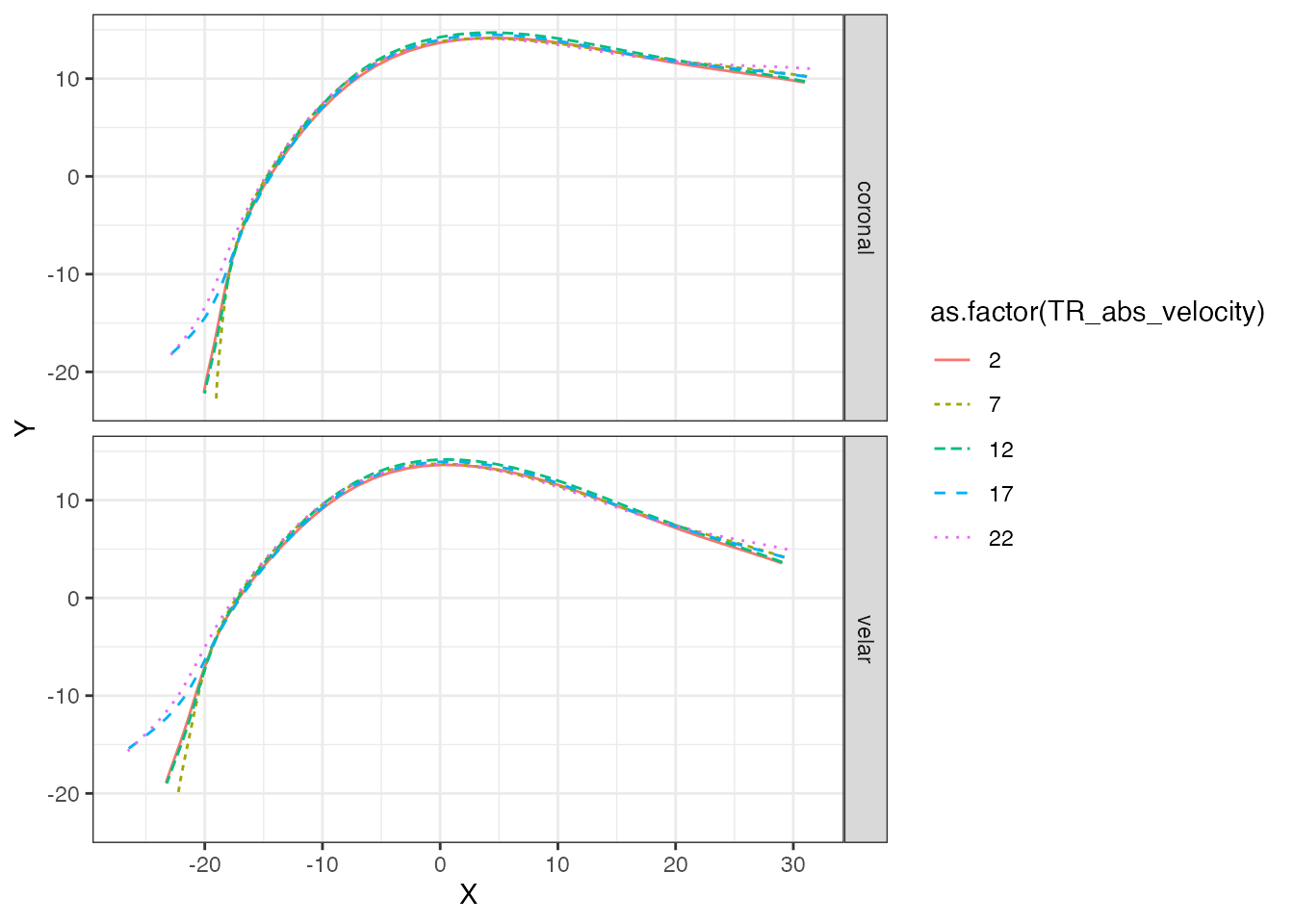

Plotting the curve with confidence intervals

If you want to add confidence intervals to the fitted curve, you have to get both the coordinates of the fitted curves using predict_polar_gam(model) and the coordinates of the confidence intervals with predict_polar_gam(model, return_ci = TRUE).

polar_multi_p <- predict_polar_gam(
  polar_multi
)

ci_data <- predict_polar_gam(
  polar_multi,
  return_ci = TRUE,
)

Now you can use the prediction dataset as the global data and the CI data with geom_polygon().

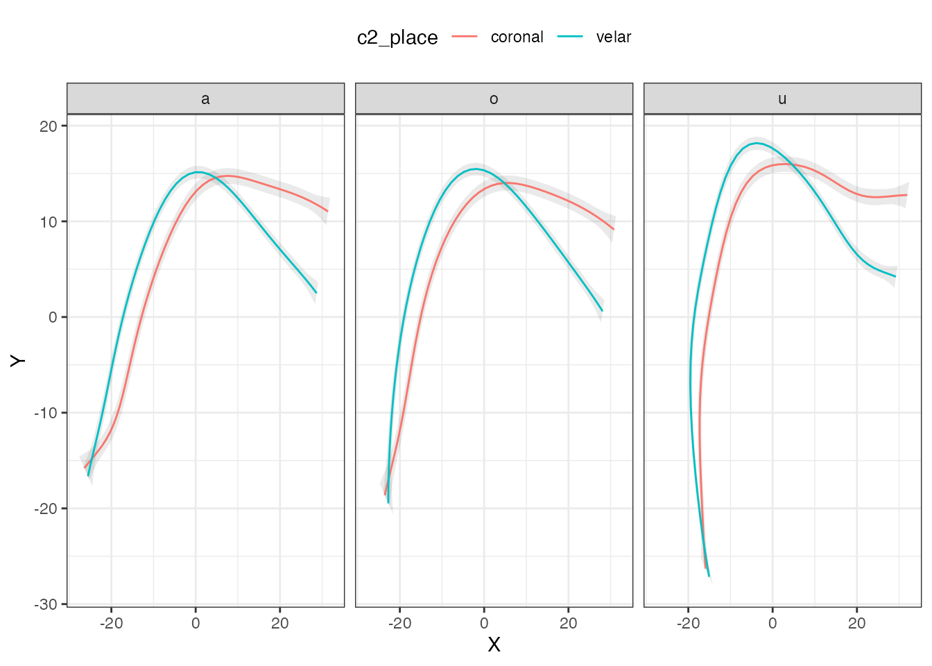
polar_multi_p %>%
  ggplot(aes(X, Y)) +
  geom_polygon(data = ci_data, aes(CI_X, CI_Y, group = c2_place), alpha = 0.1) +
  geom_path(aes(colour = c2_place)) +
  facet_grid(. ~ vowel) +
  theme(legend.position = "top")

Stefano Coretta

2022-09-04

Read data

Fit a polar GAM

Multiple predictors

Extract all predicted values

Plotting the curve with confidence intervals