Bayesian beta regressions with brms in R: A tutorial for phoneticians
Abstract
Phonetic research frequently involves analyzing numeric continuous outcome variables, such as durations, frequencies, loudness, and ratios. Another commonly used outcome type is proportions, including measures like the proportion of voicing during closure, gesture amplitude, and nasalance. Despite their bounded nature, proportions are often modeled using Gaussian regression, largely due to the default settings of commonly used statistical functions in R (e.g., lm() and lmer() from lme4). This practice persists in teaching and research, despite the fact that Gaussian models assume unbounded continuous data and may poorly fit proportion data. To address this issue, this tutorial introduces beta regression models, a more appropriate statistical approach for analyzing proportions. The beta distribution provides a flexible framework for modelling continuous data constrained between 0 and 1. The tutorial employs the brms package in R and assumes familiarity with regression modeling but no prior knowledge of Bayesian statistics. The tutorial includes two case studies illustrating the practical implementation of Bayesian beta regression models. Data and code are available at https://github.com/stefanocoretta/beta-phon.
Keywords
acoustics, articulation, proportions, Bayesian regressions, beta distribution
Introduction
Phonetic research often involves numeric continuous outcome variables, like durations, frequencies, loudness and ratios (Abramson and Whalen, 2017; Coretta et al., 2023; Gick et al., 2013; Johnson, 2003; Kluender et al., 1988; Ladefoged and Johnson, 2014; Roettger et al., 2018; Rosen, 2005). Another commonly employed type of outcome variable is data that is bounded between 0 and 1: for example, proportion of voicing during closure (Davidson, 2016), vocal folds contact quotient (Herbst et al., 2017), gesture amplitude (Carignan, 2021), nasalance (Carignan, 2021), and data from slider answers where participants can indicate responses for qualities.
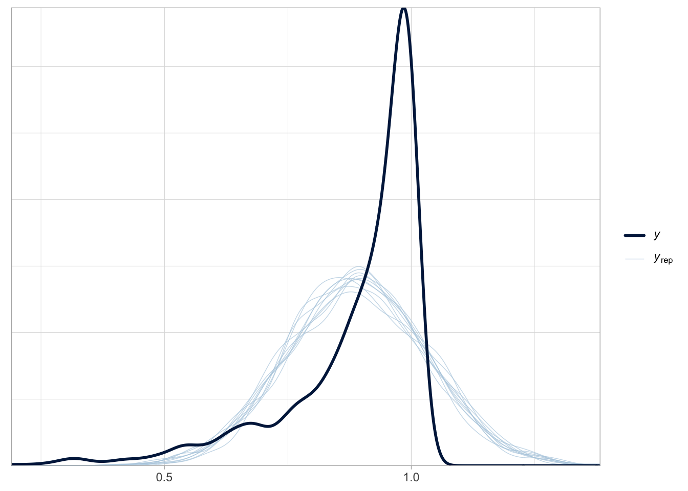
Regression models (and extensions like generalised additive models) have become a de facto standard for the statistical analysis of a variety of measures in phonetic research (Kirby and Sonderegger, 2018; Politzer-Ahles and Piccinini, 2018; Tavakoli et al., 2024). However, there is a tendency for researchers to use Gaussian distribution families (i.e. probability distributions for the outcome variable) for any measure that is numeric, irrespective of whether the measure is unbounded, like in truly Gaussian variables, or bounded, like in proportions. A possible reason is that the base R function for fitting regression models, lm(), and the lme4 function used to fit regression models with varying terms, lmer() from lme4 (Bates et al., 2015), both fit Gaussian regressions by default and the user does not have to specify the distribution family. This tacit default of using Gaussian models is also reflected in teaching practices, where significance test and models using the Gaussian distribution are the first to be taught (Baayen, 2008; Winter, 2020), due to their relative simplicity and the fact that regression models with other families are conceptual generalisations of Gaussian regression models. Figure 1 shows how poorly a Gaussian regression model fits beta-distributed data: the dark blue line is the density of data simulated to be distributed according to a beta distribution; the light blue lines are predicted distributions as generated by a Gaussian model of the data. The predicted Gaussian distributions over-predict values between 0.5 and 0.75 and under-predict values between 0.75 and 1. Furthermore, a Gaussian distribution predicts values above 1, which are not possible given the bounded nature of the data. Moreover, the density peak (median) of the Gaussian distributions is lower than the peak in the original data.
While most researchers approach proportions with Gaussian regression models, proportion are not Gaussian by nature, since they are continuous variables bounded between 0 and 1. Thus, regression models with proportions as outcome variable should be fitted using a likelihood family that assumes such unit interval data. A common and flexible distribution for this purpose is the beta distribution. Note that the beta distribution supports variables in the interval (0, 1), i.e. excluding 0 and 1; variables in the interval [0, 1], including 0 and 1, can be modelled with zero and zero/one inflated beta distributions (see Section 2). This tutorial introduces researchers to beta regression models in R using the package brms. Familiarity with regression modelling in R with a package like lme4 is assumed, but no prior knowledge of Bayesian statistics is necessary. The rest of the paper is structured as follows: Section 2 introduces the mathematical underpinnings of the beta distribution, Section 3 provides the readers with a brief explanation and justification of Bayesian regression models, while Section 4 and Section 5 illustrate how to fit Bayesian beta regression models with two case studies. The research compendium with data and code can be found at https://github.com/stefanocoretta/beta-phon.
The beta distribution
The beta distribution is often considered as the distribution for the modelling of unit interval data, i.e. data that are in the interval [0, 1] (Cribari-Neto and Zeileis, 2010a; Ferrari and Cribari-Neto, 2004). It has been extensively studied theoretically (Espinheira et al., 2008; Gupta and Nadarajah, 2014; Krysicki, 1999) and is used a baseline to compare other unit interval distributions against (Bonat et al., 2013; Kieschnick and McCullough, 2003; López, 2013). Specifically in Bayesian regression models, it was shown to perform well across a wide range of scenarios (Scholz and Bürkner, 2025, 2023), which is why we focus on the beta distribution in this tutorial.
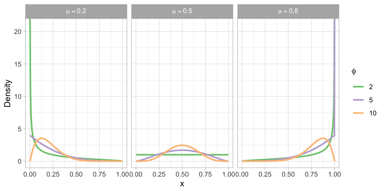
We use a common mean parametrisation for the beta distribution with mean parameter \(\mu\), bounded between 0 and 1, and positive precision parameter \(\phi\) that is roughly proportional to the inverse of the variance (\(\text{Var}(y) = \frac{\mu \, (1 - \mu)}{\phi + 1}\)).1 That is, the larger \(\phi\) the smaller the variance of the corresponding beta distribution. While the mathematical details are not needed to understand the content of this tutorial, we still write down the density below for reasons of completeness:
\[ p(y \mid \mu, \phi) = \frac{1}{B(\mu \, \phi, \; (1-\mu) \, \phi)} \; y^{\mu \, \phi -1} \; (1-y)^{(1-\mu) \, \phi -1}, \]
where \(B\) is the Beta function, a complex integral for whose numerical approximation efficient algorithms exist in every programming language. See Figure 2 for an illustration of different beta distributions based on various \(\mu\) and \(\phi\) values.
As mentioned earlier, the beta distribution handles data in the interval (0, 1), thus excluding 0 and 1. To model [0, 1] data (including 0 and 1), the zero and zero/one inflated extensions of the beta distribution can be used. Both of these are supported in the software used in this tutorial, but will not be treated here. We refer readers to (Heiss, 2021). An alternative is to use the extended-support beta family (xbeta in brms). For information on the extended-support beta family, see (Kosmidis and Zeileis, 2024).
Bayesian regression models
Bayesian regression models are being increasingly adopted within phonetics and language research more broadly (Nalborczyk et al., 2019; Vasishth et al., 2018; Verissimo, 2021). Bayesian inference involves updating of prior probability distributions in light of evidence from data, to produce posterior probability distributions. In Bayesian regression models, model parameters are modelled as full probability distributions, rather than point estimates as in Null Hypothesis Significance Testing. Given the difficulty of analytical solutions of model equations, Bayesian regressions rely on sampling algorithms to reconstruct the posterior distributions. The statistical language Stan (Stan Development Team, 2017) employs efficient and robust Markov Chain Monte Carlo algorithms for fitting a variety of models, and the R package brms allows R users to interface with Stan from within R to fit Bayesian regression models (Bürkner, 2021, 2018, 2017).
The main practical advantage of Bayesian regression models over maximum-likelihood-based frequentist regression models, like those fitted with the lme4 package (Bates et al., 2015), is that Bayesian regression models don’t suffer from the convergence issues that models fitted in lme4 (Bates et al., 2015) and other packages (Cribari-Neto and Zeileis, 2010b) that fit frequentist models do, independent of sample size. A second, long-term advantage is that Bayesian regression models allow researchers to statistically re-use information from previous studies by specifying informative priors. While prior specification is one of the main features of Bayesian inference, in this tutorial we will use the default priors as set by brms. These are sensible priors estimated from the data that facilitate convergence but bear virtually no influence on the estimated posteriors. Specifying priors requires a great deal of precise quantitative knowledge, which in some areas of phonetics is difficult to determine, so that using the default priors provided by brms is, for the purposes of this article (and initial analyses), an acceptable practice. For practical guidance on prior specification and prior predictive checks, see (Bockting et al., 2024), (Mikkola et al., 2024), (Stan Development Team, 2025) and (McElreath, 2020, pp. 82–84).
The output of Bayesian regression models is (posterior) probability distributions for the model parameters, through which researchers can quantify (un)certainty. When obtaining the summary of the posterior probability distributions, the mean and standard deviation of the posterior distribution, together with Bayesian Credible Intervals are given for each parameter. The mean and standard deviation are commonly used metrics, given that posteriors tend to be approximately Gaussian. An alternative are the median and the median absolute deviation, which can be obtained by setting robust = TRUE in summary() (note that the nature of the posterior distribution of the parameters is not related to the nature of the distribution family chosen for the outcome, so while the outcome is modelled with a beta distribution, the posteriors of the parameters follow a symmetric distribution due to the central limit theorem). Bayesian Credible Intervals (CrIs) can be calculated from the posterior distributions at several probability levels (e.g. 95, 90, 80, 60%) for a more complete view on estimated parameters. Bayesian CrIs indicate that, at a certain probability level, the parameter’s estimate lies within that interval: so, for example, a 90% CrI [A, B] indicates that there is a 90% probability that the estimate is between A and B. Different probability levels correspond to different levels of confidence: the higher the probability the higher the confidence (always conditional on data and model). Readers interested in a full and accessible exposition of Bayesian statistics are referred to (McElreath, 2019). Shorter introductions can be found in (Etz et al., 2018), (Vasishth et al., 2018) and (Nalborczyk et al., 2019).
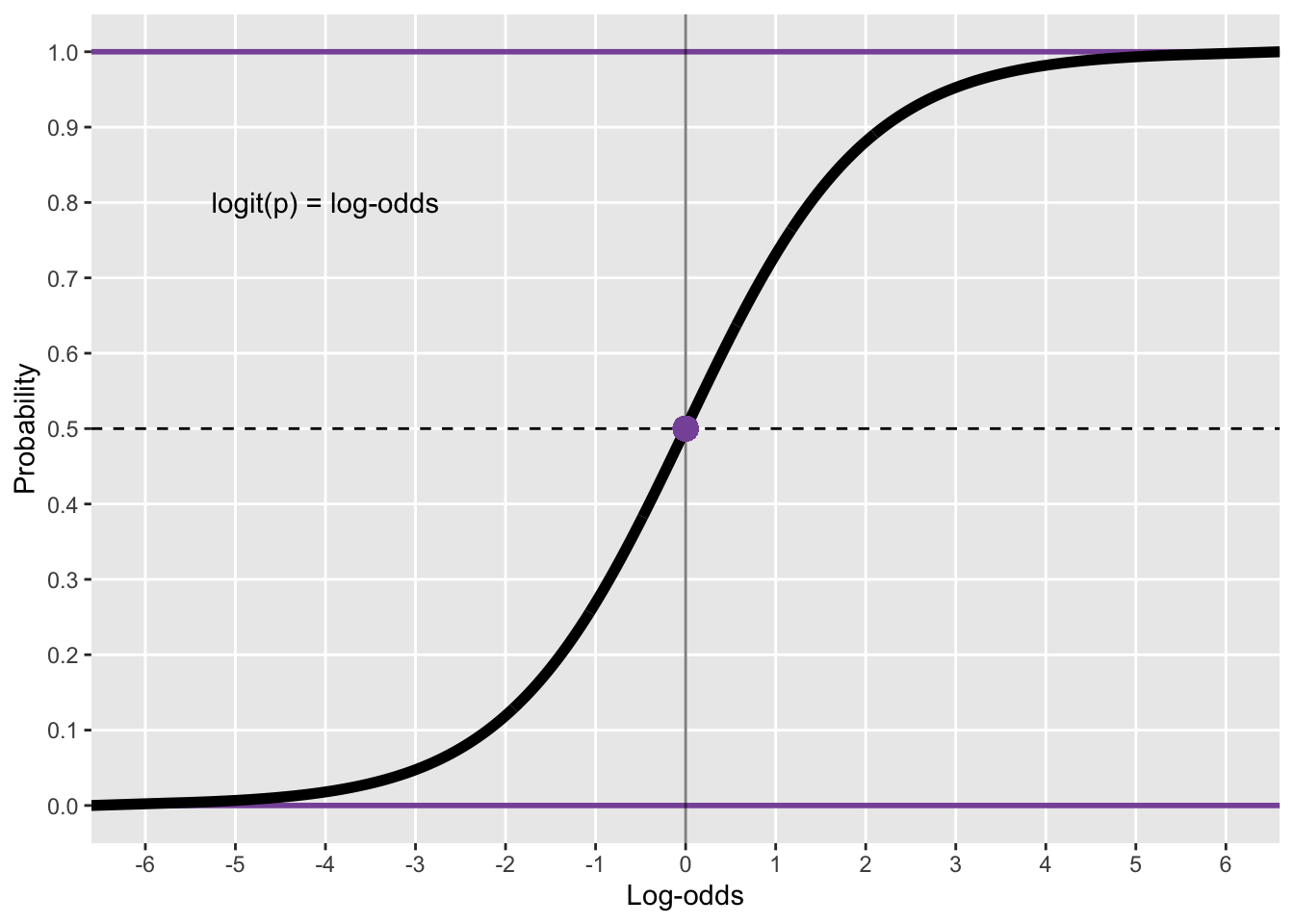
Beta regression models return coefficient estimates in log odds, similarly to Bernoulli/binomial (aka logistic) regression models. Log odds correspond to the logarithm of the odds \(\log\left(\frac{p}{1 - p}\right)\). To convert log odds into probabilities (or into a variable in the [0, 1] interval), the inverse logit function is used \(\frac{1}{1 + e^{-x}}\), where \(x\) is the log-odds value. Figure 3 illustrates the correspondence between log odds and the [0, 1] values. In R, the inverse logit can be obtained with the base R function plogis(), while the logit can be obtained with the base R function qlogis(). Another relevant transformation of log odds is exponentiation (with base R exp()) which returns the corresponding odds ratio: odds ratios indicate the rate of change in the values of the outcome variable relative to a baseline. An odds ratio of 1 indicates no change, positive odds ratios indicate an increase, while negative odds ratios correspond to a decrease. For example, if the odds ratio of the duration of /a/ vs the duration of /i/ is 1.2, this means that the duration of /a/ is grater than that of /i/. Moreover, odds ratios can be interpreted as percentage change: an odds ratio of 1.2 corresponds to a 20% increase relative to the baseline, an odds ratio of 0.8 corresponds to a 20% decrease relative to the baseline, while an odds ratio of 1 means a 0% change (i.e. no change).
Case study 1: coarticulatory voicing within consonant closure
For the first case study, we will model the proportion of coarticulatory progressive voicing within the consonant closure of voiceless stops. The measurements come from a data set of audio and electroglottographic (EGG) recordings of 19 speakers of Northwestern Italian (Coretta, 2020, 2019). The participants read frame sentences which included target words of the form /CVCo/, where C was either /k, t, p/ in all permutations and V was either /i, e, a, o, u/ (two resulting words, /peto/ and /kako/ were excluded because they are profanities), for a total of 43 target words. There were 4 different frame sentence: Scrivete X sul foglio ‘Write X on the sheet’, Ha detto X sei volte ‘She said X six times’, Sentivo X di nuovo ‘I heard X again’, Ripete X da sempre ‘She’s been repeating X since ever’. There is a total of 172 trials per participant (3,268 grand total). The actual observation count is 2,419, after removing speech errors, EGG measurement errors, and cases in which voicing ceased before the closure onset/after the closure offset of the second consonant in the target word.
The proportion of voicing during the closure of the second consonant was calculated as the proportion of contiguous voicing duration after closure onset to total duration of closure. The following code chunk attaches the tidyverse packages (for reading and wrangling data, Wickham et al., 2019) and loads the ita_egg tibble (data frame). The tibble is filtered so as to remove voicing proportions (voi_clo_prop) that are smaller than 0 and greater than 1. The variables vowel (first vowel in the target word) and c2 (second consonant in the target word) are converted to factors to specify the order of the levels. Table 1 shows the first ten rows of the tibble (only relevant columns are included).
# attach tidyverse and set light theme for plots
library(tidyverse)
theme_set(theme_light())

# load tibble
load("data/coretta2018/ita_egg.rda")

# filter and mutate data
ita_egg <- ita_egg |>
  filter(voi_clo_prop > 0, voi_clo_prop < 1) |>
  mutate(
    vowel = factor(vowel, levels = c("i", "e", "a", "o", "u")),
    c2 = factor(c2, levels = c("k", "t", "p"))
)| speaker | word | vowel | c2 | voi_clo_prop |
|---|---|---|---|---|
| it01 | poto | o | t | 0.0457950 |
| it01 | topo | o | p | 0.3522513 |
| it01 | pato | a | t | 0.1440749 |
| it01 | teto | e | t | 0.3610916 |
| it01 | toto | o | t | 0.2743519 |
| it01 | puco | u | k | 0.1943984 |
| it01 | chipo | i | p | 0.2227896 |
| it01 | peco | e | k | 0.1835596 |
| it01 | poco | o | k | 0.1771007 |
| it01 | poto | o | t | 0.1525163 |
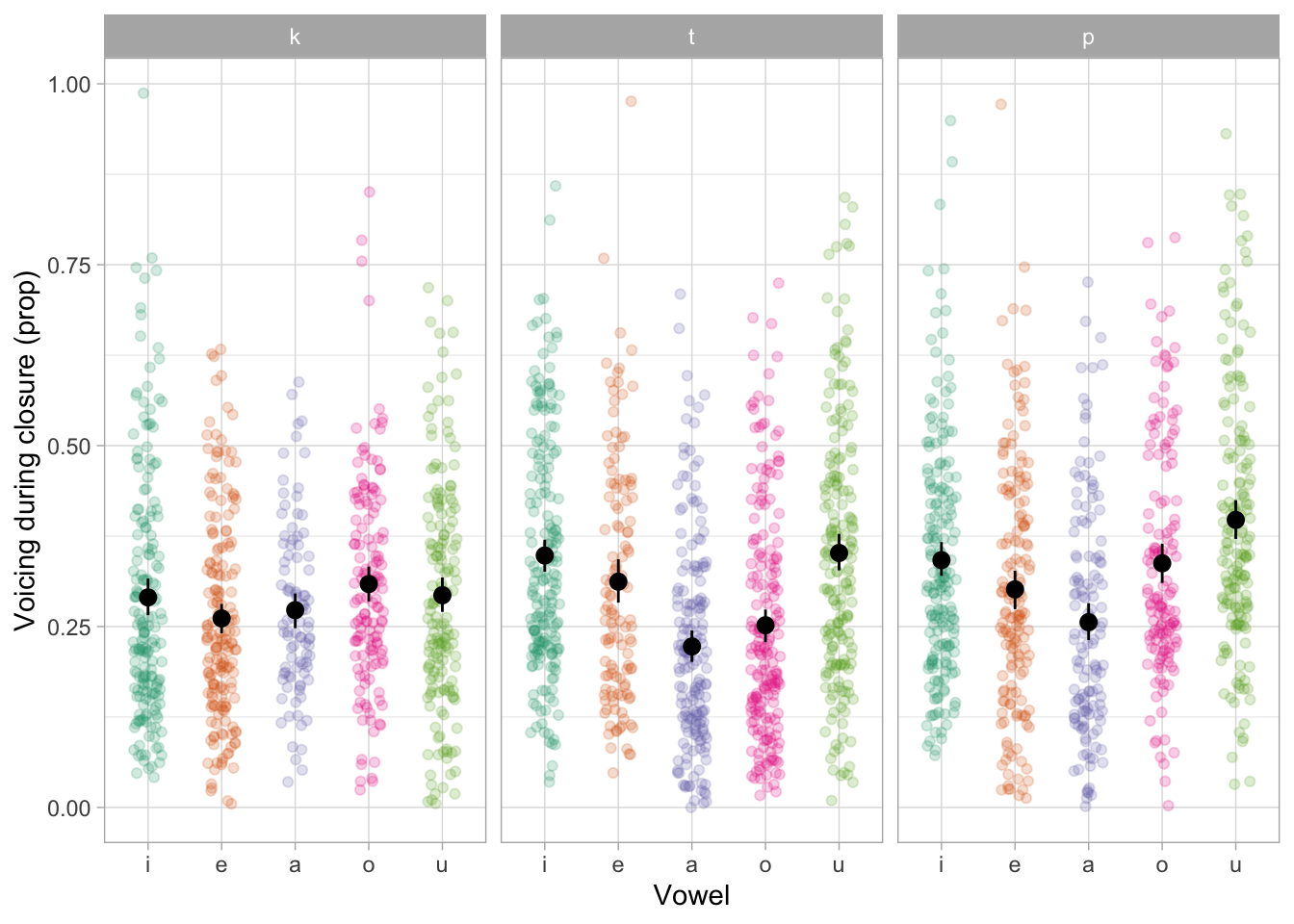
Figure 4 shows the raw voicing duration proportion values split by vowel /i, e, a, o, u/ and second consonant /k, t, p/ in the /CVCo/ target words. The plot suggests that, on average, the voicing proportion is slightly lower with /k/ than with /t, p/. Moreover, there is greater variability between vowels in /t, p/ than in /k/. We will use a beta regression model to assess whether the place of articulation of the consonant affects the proportion of coarticulatory progressive voicing, while averaging across vowels (of course, another question that could be answered with the same model is if different vowels lead to different voicing proportions, but for sake of space we restrict this tutorial to the former question). A general expectation is that the proportion of progressive voicing should increase with fronter places of articulation (so from /k/ to /t/ to /p/) given the aerodynamic constraints which obtain with vocal fold vibration during a fully occluded oral tract (Ohala, 2011; Rothenberg, 1967; van den Berg, 1958).
We will use brms to fit a Bayesian beta regression (Bürkner, 2017). The model has voicing proportion as the outcome variable and the following terms: an interaction between vowel (/i, e, a, o, u/) and second consonant C2 (/k, t, p/), centred speech rate (number of syllables per second); as varying (aka random) terms, we included by-speaker varying coefficients for the vowel/consonant interaction and for centred speech rate.2 The categorical predictors vowel and C2 are coded using indexing rather than the traditional R contrasts (such as treatment or sum), as advocated in (McElreath, 2019, p 155, Ch 8): in R, this corresponds to suppressing the model’s intercept with the 0 + syntax. With this approach, the model’s coefficients do not represent differences from a reference level (normally the intercept), rather they represent the predicted mean for all combinations of each categorical predictor’s levels (no contrasts are applied). The following code shows the coding matrix for a hypothetical predictor with three levels, coded using treatment contrasts and indexing.
fac <- factor(c("a", "b", "c"))

# Treatment contrasts
contrasts(fac)
b c
a 0 0
b 1 0
c 0 1# Indexing
diag(nlevels(fac)) [,1] [,2] [,3]
[1,] 1 0 0
[2,] 0 1 0
[3,] 0 0 1With indexing, a model would have one coefficient for the mean of “a”, one for the mean of “b”, and one for the mean of “c”. No comparisons between levels are present in the matrix, but these can be obtained from the model post-hoc (as we do below).
One benefit of using indexing is that uncertainty is equally distributed across all levels of categorical predictors, since priors apply on the mean of each level, rather than on the difference of subsequent levels from the reference level. The latter scenario, which applies in traditional contrasts, including treatment and sum, makes estimates of the last level in the predictor more uncertain than the estimates of the other levels, given that the uncertainty of the intercept is added to the uncertainty of the difference. As explained in Section 3, using the default priors calculated by brms is an acceptable method in the absence of very specific quantitative expectation, given that the default priors are weak enough to bear little effect on posteriors. Researchers should use their own judgement and expertise in a case by case fashion.
# attach brms
library(brms)

# fit the model
# Takes 3 minutes on MacBook Pro 2020, M1
voi_prop_bm <- brm(
  # model formula
  voi_clo_prop ~
    # constant terms
    0 + vowel:c2 + speech_rate_c +
    # varying terms
    (0 + vowel:c2 + speech_rate_c | speaker),
  # uses the beta family for the outcome
  family = Beta,
  data = ita_egg,
  cores = 4,
  seed = 3749,
  file = "data/cache/voi_prop_bm"
)
The summary() function prints the full model summary. For conciseness, we will use the fixef() function which prints the regression coefficients. Table 2 reports the output of fixef() as a table (we round all values to the nearest 2 digits for clarity.). For each coefficient in the model, fixef() prints the name of the coefficient, the mean estimate (i.e. the mean of the posterior distribution calculated from the MCMC draws), the estimate error (i.e. the standard deviation of the posterior distribution) and the lower and upper limits of a Bayesian Credible interval (CrI) of the posterior distribution. Note that all values are in log odds, since the link function in beta regressions is the logistic function, like in binomial/Bernoulli regressions. Here, we print an 80% CrI. There is nothing special about 95% CrI within Bayesian inference and instead experts recommend to check and report a variety of CrIs. Obtaining CrIs at different probability levels allows researchers to make more fine-grained inferential statements than the frequentist significance dichotomy affords. For simplicity of exposition, we will use 80% CrIs in this case study but we strongly recommend researchers to always obtain CrIs at different levels of probability and base their inferences on all and not one in particular. To reiterate, in Bayesian inference, an 80% CrI indicates the range of values within which the true estimate falls at 80% probability or confidence.
fixef(voi_prop_bm, prob = c(0.1, 0.9))voi_prop_bm).
| Estimate | Est.Error | Q10 | Q90 | |
|---|---|---|---|---|
| speech_rate_c | 0.08 | 0.06 | 0.01 | 0.15 |
| voweli:c2k | -0.91 | 0.14 | -1.08 | -0.74 |
| vowele:c2k | -1.08 | 0.11 | -1.22 | -0.94 |
| vowela:c2k | -0.99 | 0.12 | -1.14 | -0.84 |
| vowelo:c2k | -0.79 | 0.14 | -0.96 | -0.62 |
| vowelu:c2k | -1.00 | 0.16 | -1.20 | -0.80 |
| voweli:c2t | -0.66 | 0.11 | -0.79 | -0.53 |
| vowele:c2t | -0.84 | 0.14 | -1.02 | -0.66 |
| vowela:c2t | -1.43 | 0.13 | -1.60 | -1.26 |
| vowelo:c2t | -1.15 | 0.13 | -1.31 | -0.99 |
| vowelu:c2t | -0.68 | 0.12 | -0.83 | -0.54 |
| voweli:c2p | -0.68 | 0.11 | -0.81 | -0.54 |
| vowele:c2p | -0.88 | 0.15 | -1.07 | -0.68 |
| vowela:c2p | -1.14 | 0.13 | -1.31 | -0.98 |
| vowelo:c2p | -0.66 | 0.11 | -0.80 | -0.53 |
| vowelu:c2p | -0.44 | 0.12 | -0.59 | -0.28 |
From the summary, we see that speech rate (number of syllables per second) has a positive effect on voicing proportion: the 80% CrI is between 0.01 and 0.15 log odds [\(\beta\) = 0.08, SD = 0.06]. Log odds can be converted to odds ratios by exponentiating the value: 0.01-0.15 log odds correspond to an odds ratio of 1.01 to 1.16, or as percentages, to an increase of voicing of 1 to 16% for every increase of one syllable per second. Since this is an 80% CrI, we can be 80% confident that the true effect of speech rate is between 1-16% increase of voicing proportion, conditional on the data and model. Note that transforming measures this way is appropriate only with quantile-based measures (like CrIs) but not with moments like the mean and standard deviation: to correctly get mean and SDs in the transformed scale, you must first extract the posterior draws (see below), convert them and then take moments such as mean and SD (for a more detailed explanation, see Bürkner, 2025, p. 101). In the avoidance of doubt, we will always transform the drawn values first and then take summary measures.
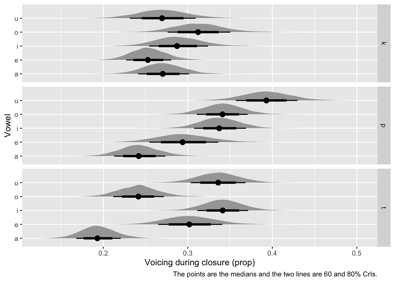
Turning now to the coefficients for vowel and C2, given the indexing approach of coding these variables the model summary and the output of fixef() reports the predictions in log odds for each combination of vowel and C2, rather than differences between levels. The posteriors of the coefficients for vowel and C2 are the estimated \(\mu\)s of the beta distribution, since the beta distribution is parametrised with \(\mu\) and \(\phi\). We will not discuss \(\phi\), although the estimate of this parameter can be found in the summary of the model, under “Further Distributional Parameters”.The CrIs of the vowel/C2 coefficients span all negative log-odds values: these correspond to proportions that are lower than 0.5 (which is 0 in log odds). This matches the general trends in the raw data, which we plotted in Figure 4. Next, we will plot the predicted proportions of each vowel/C2 combination at mean speech rate (i.e. centred speech rate = 0) and then calculate the average pair-wise difference in voicing proportion between /k, t, p/.
Before being able to plot the predictions, it’s important to get familiar with the so-called posterior draws. Bayesian regression models are fitted using Markov Chain Monte Carlo (MCMC) methods, as briefly explained in Section 3. The brm() function runs four MCMC chains with 2000 iterations each by default. These are sufficient in most cases. The first 1000 iterations of each chain are used for “warmup”, where the MCMC algorithm is optimised to find the posterior probability. The second half of the iterations, 1000 per chain, are used for sampling from the posterior probability. Each iteration returns a drawn value for each parameter in the model. The list of values drawn during the Monte Carlo sampling are called the “posterior draws”. Since four chains are run, a total of 4000 posterior values are generated. The posterior draws are used for inference: we can plot them, summarise them, transform them and combine them in any way to answer specific questions.
Posterior draws can be conveniently obtained with the as_draws_df() from brms. For the moment, we will extract only the draws of the constant (aka fixed) regression coefficients (model variables starting with b_). To check which coefficients are available in a model, use get_variables() from the tidybayes package (Kay, 2019). as_draws_df() returns a tibble where each column contains the drawn values of a coefficient. Table 3 shows the first ten rows and first five columns of the output of as_draws_df(). The probability distribution of the drawn values of each coefficient is the posterior probability distribution of that coefficient. Note that, due to the indexing coding of vowel and C2, all coefficient except b_speech_rate_c are drawn log-odds values for each vowel/C2 combination (the drawn values for b_speech_rate_c are drawn differences in log-odds values for each unit increase of speech rate). The drawn values are in log odds, but we can convert them to proportions with plogis() (we will do this when plotting below).
# extract only coefficient variables starting with "b_"
voi_prop_bm_draws <- as_draws_df(voi_prop_bm, variable = "^b_", regex = TRUE)voi_prop_bm.
| b_speech_rate_c | b_voweli:c2k | b_vowele:c2k | b_vowela:c2k | b_vowelo:c2k |
|---|---|---|---|---|
| 0.1593890 | -0.7213516 | -1.046577 | -1.1197185 | -1.0191525 |
| 0.0351033 | -0.7492306 | -1.385450 | -1.0633164 | -0.8854320 |
| 0.1259352 | -0.8472495 | -0.975776 | -1.0972735 | -0.6440836 |
| 0.0640492 | -0.7033469 | -1.068626 | -1.0475190 | -0.8328252 |
| 0.0319081 | -0.7659281 | -1.177656 | -0.9357499 | -0.6955130 |
| 0.0729965 | -0.8494392 | -1.226692 | -1.0635364 | -0.7692243 |
| 0.1009609 | -0.9546148 | -1.072955 | -1.1408255 | -0.8566750 |
| 0.0735392 | -1.0160675 | -1.065025 | -1.1736263 | -0.8334884 |
| 0.0870061 | -1.0436475 | -1.069337 | -1.2632061 | -0.7941857 |
| 0.0923815 | -1.2042168 | -1.041238 | -0.9158689 | -0.6444492 |
We can now wrangle this tibble and plot the posterior distributions for each vowel/C2 combination. Table 4 shows the first ten rows.
voi_prop_bm_draws_long <- voi_prop_bm_draws |>
  # drop b_speech_rate_c before pivoting
  select(-b_speech_rate_c) |>
  # pivot vowel:c2 columns
  pivot_longer(`b_voweli:c2k`:`b_vowelu:c2p`, names_to = "coeff") |>
  # separate "coeff" labels into type ("b"), vowel and c2
separate(coeff, into = c("type", "vowel", "c2"))voi_prop_bm in long format.
| .chain | .iteration | .draw | type | vowel | c2 | value |
|---|---|---|---|---|---|---|
| 1 | 1 | 1 | b | voweli | c2k | -0.7213516 |
| 1 | 1 | 1 | b | vowele | c2k | -1.0465766 |
| 1 | 1 | 1 | b | vowela | c2k | -1.1197185 |
| 1 | 1 | 1 | b | vowelo | c2k | -1.0191525 |
| 1 | 1 | 1 | b | vowelu | c2k | -1.0523007 |
| 1 | 1 | 1 | b | voweli | c2t | -0.6248875 |
| 1 | 1 | 1 | b | vowele | c2t | -0.7951552 |
| 1 | 1 | 1 | b | vowela | c2t | -1.3999773 |
| 1 | 1 | 1 | b | vowelo | c2t | -1.0950180 |
| 1 | 1 | 1 | b | vowelu | c2t | -0.6682030 |
For plotting, we can use ggplot2 statistics layers from the ggdist package [(Kay, 2023); kay2024]. stat_halfeye() plots the density of the posterior probability (in grey), its median (point) and CrIs (lines). Let’s use 60 and 80% CrIs and transform the log-odds values to proportions with plogis(). See Figure 5.
# attach ggdist package
library(ggdist)

voi_prop_bm_draws_long |>
  mutate(
    c2 = str_remove(c2, "c2") |> factor(levels = c("k", "t", "p")),
    vowel = str_remove(vowel, "vowel")
  ) |>
  ggplot(aes(plogis(value), vowel)) +
  stat_halfeye(.width = c(0.6, 0.8)) +
  facet_grid(rows = vars(c2)) +
  labs(
    caption = "The points are the medians and the two lines are 60 and 80% CrIs.",
    x = "Voicing during closure (prop)",
    y = "Vowel"
  )
voi_prop_bm.
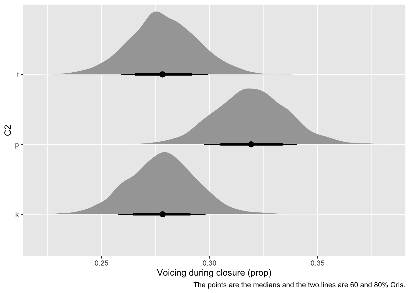
What if we want to plot the average predicted voicing proportion for the three consonants /k, t, p/? We can “marginalise” over vowel, i.e. take the mean across vowels within each consonant for each posterior draw, and the posterior distribution of the resulting list of values is the predicted posterior distribution of voicing proportion for each consonant, assuming an “average” vowel. See Figure 6 for the density of these posteriors. For a detailed treatment of various approaches to marginalisation that apply to more complex cases like those involving numeric predictors, see (Arel-Bundock et al., 2024).
voi_prop_bm_draws_long_c2 <- voi_prop_bm_draws_long |>
  # grouping by .draw and c2 ensures that averaging applies only within draw and c2
  group_by(.draw, c2) |>
  # calculate the mean value within draw/c2
  summarise(
    value_mean = mean(value), .groups = "drop"
  )
voi_prop_bm_draws_long_c2 |>
mutate(
c2 = str_remove(c2, "c2") |> factor(levels = c("k", "t", "p"))
) |>
ggplot(aes(plogis(value_mean), c2)) +
stat_halfeye(.width = c(0.6, 0.8)) +
labs(
caption = "The points are the medians and the two lines are 60 and 80% CrIs.",
x = "Voicing during closure (prop)",
y = "C2"
)
Based on the expected posterior distributions of the mean voicing proportion by consonant, /p/ has a somewhat higher voicing proportion than /k/ and /t/. The real question is: how much higher? We can quantify this by taking the difference of the drawn values for /p/ and those for /k, t/ (all averaged across vowels). Since we want to compare /k, t/ with /p/, we should first average the average draws of /k, t/ and then take the difference of the averaged /k, t/ draws and the draws of /p/. Table 5 shows the first ten rows of the resulting data frame. The posterior distribution of the expected difference is shown in Figure 7.
voi_prop_bm_diff <- voi_prop_bm_draws_long_c2 |>
  # pivot data to create one column per consonant with the mean drawn values,
  # with one draw per raw
  pivot_wider(names_from = c2, values_from = value_mean) |>
  mutate(
    # calculate the mean of /k/ and /t/, for each draw
    c2tk = mean(c(c2k, c2t)),
    # calculate the difference of /p/ and /k, t/
    c2p_tk_diff = c2p - c2tk
)| .draw | c2k | c2p | c2t | c2tk | c2p_tk_diff |
|---|---|---|---|---|---|
| 1 | -0.9918200 | -0.7450832 | -0.9166482 | -0.9533426 | 0.2082595 |
| 2 | -1.0240673 | -0.7904348 | -1.0322325 | -0.9533426 | 0.1629079 |
| 3 | -0.8954946 | -0.6873228 | -0.8904412 | -0.9533426 | 0.2660199 |
| 4 | -0.9442361 | -0.8135191 | -0.9095122 | -0.9533426 | 0.1398235 |
| 5 | -0.9278262 | -0.7908457 | -0.9200903 | -0.9533426 | 0.1624970 |
| 6 | -0.9825895 | -0.7283054 | -0.9262196 | -0.9533426 | 0.2250372 |
| 7 | -1.0482359 | -0.8731592 | -1.0841208 | -0.9533426 | 0.0801835 |
| 8 | -1.0613713 | -0.8751219 | -1.0741555 | -0.9533426 | 0.0782208 |
| 9 | -1.0622522 | -0.9739388 | -1.0481834 | -0.9533426 | -0.0205962 |
| 10 | -0.9293998 | -0.8287910 | -0.9526105 | -0.9533426 | 0.1245517 |
voi_prop_bm_diff |>
  ggplot(aes(c2p_tk_diff)) +
  stat_halfeye(.width = c(0.6, 0.8, 0.9)) +
  geom_vline(xintercept = 0) +
  labs(
    x = "Log-odds difference in /p/ vs /k, t/",
    y = element_blank()
  )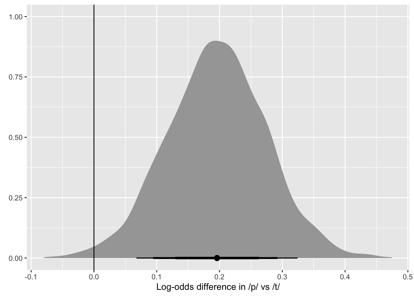
Once we have the posterior difference, we can obtain CrIs of the difference using quantile2() from the posterior package (Bürkner et al., 2024). Beware that the values of the difference are in log odds! We can convert these into odds ratios with exp(). The output of the code below is shown in Table 6. Odds ratios indicate the ratio of the difference between A and B, so that 1 means no difference, values greater than 1 indicate an increase in A relative to B and values lower than 1 indicate a decrease in A relative to B. Odds ratios are useful when looking at differences that are in log odds because while the relative magnitude of the difference in proportion between two groups is the same independent of the baseline proportion, the absolute magnitude of the difference depends on the baseline value. For example, an odds ratio difference of 1.25 would correspond to a proportion increase of about 3 percentage points if the baseline proportion is 0.62 but it would correspond to a proportion increase of 5 percentage points if the baseline proportion is 0.73 and 1 percentage point if the baseline is 0.99. Of course, in real research contexts it is still useful to think about absolute magnitudes and their relevance from a conceptual and methodological perspective. In this tutorial we just focus on odds ratios for simplicity.
library(posterior)

voi_bm_quant <- voi_prop_bm_diff |>
  mutate(c2p_tk_diff_ratio = exp(c2p_tk_diff)) |>
  reframe(
    # 90% CrI
    q90 = quantile2(c2p_tk_diff_ratio, probs = c(0.05, 0.95)),
    # 80% CrI
    q80 = quantile2(c2p_tk_diff_ratio, probs = c(0.1, 0.9)),
    # 60% CrI
    q60 = quantile2(c2p_tk_diff_ratio, probs = c(0.2, 0.8)),
  ) |>
  # round to 2 digits
mutate(across(everything(), ~round(.x, 2)))| q90 | q80 | q60 |
|---|---|---|
| 1.07 | 1.10 | 1.14 |
| 1.38 | 1.34 | 1.30 |
Based on the model and data, there is a 90% probability that the voicing proportion in /p/ is 1.07-1.38 times longer (or 7-38% increase) than in /k, t/. At 80% confidence, the change ratio is 1.10-1.34 (or 10-34% increase) while at 60% confidence is 1.14-1.30 (14-30% increase). In other words we can be quite confident that the voicing proportion in /p/ is greater than in /k, t/ and that the increase is less than 35%. The brms package comes with a convenient function, conditional_effects(), to plot posterior means and CrIs based on predictors in the model. In Figure 8, we plot the predicted proportion of voicing by consonant and vowel.
ce <- conditional_effects(voi_prop_bm, "c2:vowel")
p <- plot(ce, plot = FALSE)[[1]]
p + labs(x = "C2", y = "Voicing during closure (prop)")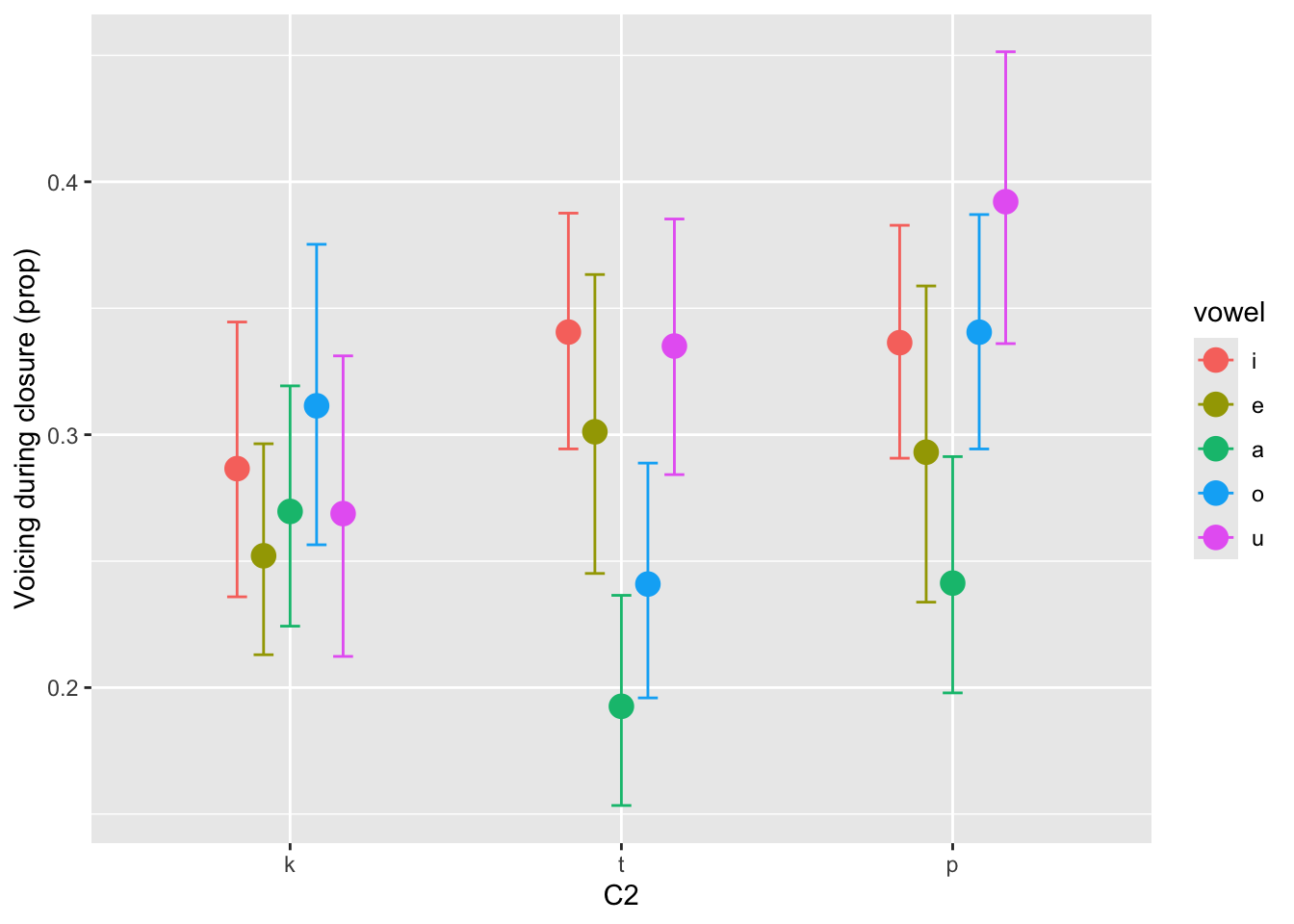
Finally, the package marginaleffects (Arel-Bundock et al., 2025) has two other convenience functions that return CrIs of comparisons across predictor levels (avg_comparisons()) and CrIs of posterior predictions across predictor levels (avg_predictions). Both functions take the model and a list of variables as arguments. Optionally, you can set the confidence level with the conf_level argument (here, we set it to 0.8, or 80%). avg_comparisons() allows the user to specify the type of comparison for each variable: here we set "pairwise" to calculate pairwise comparisons of each level of c2. The output of the two functions is shown in Table 7 and Table 8.3
library(marginaleffects)

avg_comparisons(voi_prop_bm, variables = list(c2 = "pairwise"), conf_level = 0.8, type = "link")
avg_predictions(voi_prop_bm, variables = "vowel", conf_level = 0.8)| term | contrast | estimate | conf.low | conf.high |
|---|---|---|---|---|
| c2 | p - k | 0.218 | 0.178 | 0.256 |
| c2 | p - t | 0.183 | 0.145 | 0.219 |
| c2 | t - k | 0.035 | -0.004 | 0.074 |
| vowel | estimate | conf.low | conf.high |
|---|---|---|---|
| i | 0.331 | 0.325 | 0.338 |
| e | 0.300 | 0.293 | 0.307 |
| a | 0.245 | 0.238 | 0.252 |
| o | 0.305 | 0.298 | 0.312 |
| u | 0.348 | 0.341 | 0.354 |
In sum, we used a Bayesian beta regression model to assess whether different places of articulation affect the proportion of coarticulatory progressive voicing. The expectation was that that the proportion of progressive voicing should increase with fronter places of articulation (so from /k/ to /t/ to /p/). This expectation is not borne out by the results: while the proportion of voicing is robustly greater in /p/ than in /k, t/ (at 90% probability, the voicing proportion in /p/ is 7-38% higher), the difference in voicing proportion between /k/ and /t/ is very small and uncertain.
Case study 2: coarticulatory vowel nasalisation
For the second case study we will use data from (Carignan, 2021). The study looked at properties of nasality in German VNC sequences. Here, we will focus on the effect of C voicing (voiceless /t/ vs voiced /d/) on the proportion of nasalisation within the vowel in the VNC sequence. Previous work on coarticulatory nasalisation in English has suggested that vowels followed by an NC sequence where C is voiceless (NT) should show earlier coarticulatory nasalisation than vowels followed by an NC sequence where C is voiced (ND). This pattern has been suggested to be driven by the articulatory and acoustic incompatibility of voicelessness and nasalisation, by which the velum opening gesture of the nasal consonant is pushed away (i.e. earlier) when the consonant following the nasal is voiceless (Beddor, 2009; Carignan et al., 2015; Cho et al., 2017; Fowler, 2005). Everything else being equal, a greater proportion of vowel nasalisation (from the perspective of time) should be found in vowels followed by NT than in vowels followed by ND.
We will model the proportion of coarticulatory nasalisation in the German short vowels /i, e, a, o, u/ when followed by /nt/ or /nd/, using a Bayesian beta regression model. The proportion was calculated as the proportion of the nasal interval to the duration of the vowel. The nasal interval was defined thus: the interval between the time of peak velocity of velum opening to the offset of the vowel. We will use the results of the regression model to answer the following questions:
- Is the nasalisation proportion, on average across vowels, greater in voiceless NC sequences?
- Is there individual speaker variation?
Table 9 shows the first ten rows of the data. The data contains the following columns:
speakerindicates the speaker ID.labelis the word label as given in the original data.vowelis the target vowel in the VNC sequence.NCis the NC sequence (voiceless /nt/ or voiced /nd/).voicingindicates the voicing of C.nas_propis the proportion of coarticulatory nasalisation of the vowel.
nasal <- read_csv("data/carignan2021/nasal.csv")| speaker | label | vowel | NC | voicing | nas_prop |
|---|---|---|---|---|---|
| S03 | b_U_nt@___N_B17/s | u | nt | voiceless | 0.3668820 |
| S03 | b_a_nd@___N_B19/s | a | nd | voiced | 0.1954858 |
| S03 | b_a_nt@___N_B15/s | a | nt | voiceless | 0.2786485 |
| S03 | f_I_nt@___N_B05/s | i | nt | voiceless | 0.7642259 |
| S03 | l_I_nd@___N_B06/s | i | nd | voiced | 0.0052949 |
| S03 | p_E_nt____N_B09/s | e | nt | voiceless | 0.3347331 |
| S03 | r_a_nt@___N_B06/s | a | nt | voiceless | 0.2431760 |
| S03 | v_I_nd@___N_B07/s | i | nd | voiced | 0.0247572 |
| S03 | v__I_nt_6___N_B15/s | i | nt | voiceless | 0.1350081 |
| S03 | z_E_nd@___N_B17/s | e | nd | voiced | 0.5378522 |
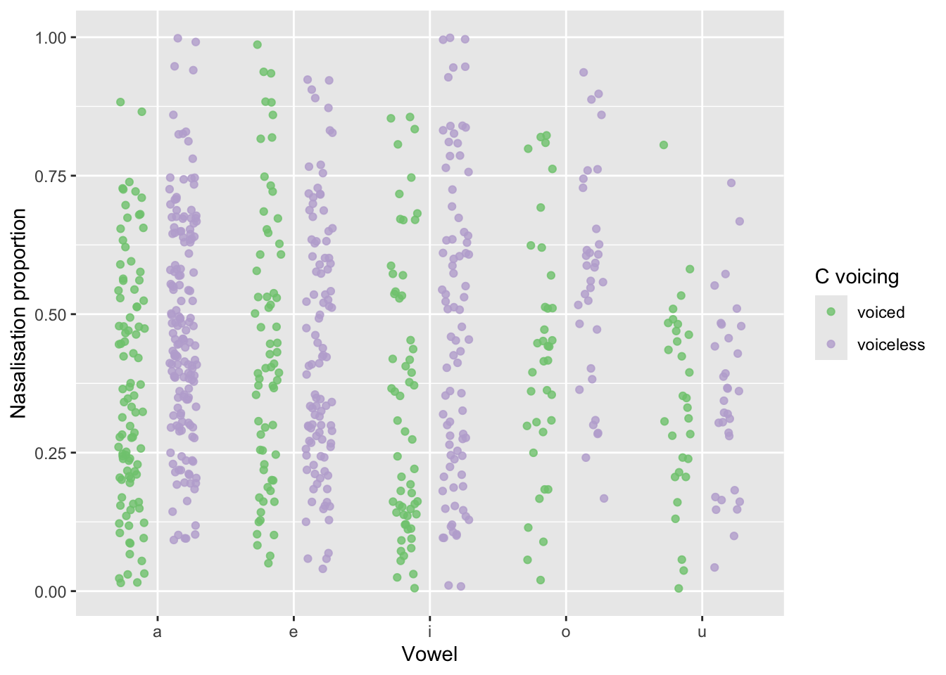
Figure 9 shows the proportion of coarticulatory nasalisation in vowels followed by /nd/ (voiced) vs /nt/ (voiceless) sequences, for the short vowels /i, e, a, o, u/. We can see a pattern of higher nasalisation proportion in vowels followed by /nt/, at least in the vowels /a, i, o/. For /e, u/, the distribution of nasalisation proportion seems to be similar between the voiced and voiceless contexts.
Now onto modelling with a beta regression. Note that a full appropriate model would include further predictors (both constant and varying), but for simplicity here we include only the following predictors: voicing (voiced /nd/ vs voiceless /nt/), vowel (/i, e, a, o, u/), including an interaction between them. As varying terms, we include a varying intercept by speaker and a by-speaker varying slope for voicing and vowel in interaction. As with the model from the first case study, voicing and vowel are coded using indexing, by suppressing the intercept with 0 +. Here’s the code of the model.
nas_prop_bm <- brm(
  nas_prop ~ 0 + voicing:vowel + (0 + voicing:vowel | speaker),
  data = nasal,
  family = Beta,
  cores = 4,
  seed = 3749,
  file = "data/cache/nas_prop_bm"
)
Let’s inspect the output of fixef(), reported in Table 10.
fixef(nas_prop_bm, prob = c(0.1, 0.9))nas_prop_bm).
| Estimate | Est.Error | Q10 | Q90 | |
|---|---|---|---|---|
| voicingvoiced:vowela | -0.61 | 0.12 | -0.77 | -0.46 |
| voicingvoiceless:vowela | -0.08 | 0.09 | -0.19 | 0.04 |
| voicingvoiced:vowele | -0.19 | 0.16 | -0.38 | 0.01 |
| voicingvoiceless:vowele | -0.25 | 0.10 | -0.38 | -0.12 |
| voicingvoiced:voweli | -0.74 | 0.19 | -0.98 | -0.51 |
| voicingvoiceless:voweli | -0.12 | 0.18 | -0.35 | 0.10 |
| voicingvoiced:vowelo | -0.34 | 0.16 | -0.54 | -0.14 |
| voicingvoiceless:vowelo | 0.25 | 0.15 | 0.05 | 0.44 |
| voicingvoiced:vowelu | -0.71 | 0.18 | -0.94 | -0.49 |
| voicingvoiceless:vowelu | -0.58 | 0.16 | -0.78 | -0.38 |
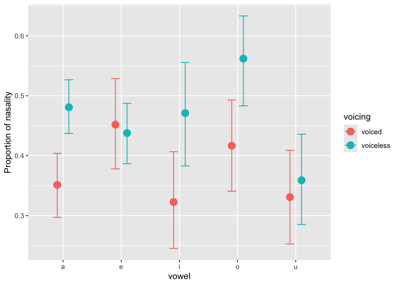
Negative log odds indicate a proportion that is smaller than 50%, while positive log odds a proportion that is greater than 50%. Generally, the expected log-odd predictions in Table 10 are negative, indicating an overall tendency for the nasalisation to take less than 50% of the duration of the vowel. Moreover, the predictions are higher for voiceless NC sequences than for voiced NC sequences, indicating a greater proportion of nasalisation in the former. However there is vowel-specific variation, and there doesn’t seem to be much of a difference in nasalisation proportion in /e/ and /u/. Figure 10 shows the expected predictions with conditional_effects(), which should make the interpretation of the predictions from Table 10 clearer.
ce <- conditional_effects(nas_prop_bm, "vowel:voicing")
p <- plot(ce, plot = FALSE)[[1]]
p +
  labs(
    y = "Proportion of nasality"
  )
Now that we fitted the model we can use the posterior draws to answer the two research questions (repeated from above):
- Is the nasalisation proportion, on average across vowels, greater in voiceless NC sequences?
- Is there individual speaker variation?
To answer question 1, we can calculate the average difference in nasalisation proportion by first calculating the average nasalisation across all vowels for voiced and voiceless sequences (see Table 11 for the output of this step) and then take the difference of those, similarly to what we have done in the case study in Section 4.
# extract only coefficient variables starting with "b_"
nas_prop_bm_draws <- as_draws_df(nas_prop_bm, variable = "^b_", regex = TRUE)

nas_prop_bm_draws_long <- nas_prop_bm_draws |>
  # pivot vowel:c2 columns
  pivot_longer(`b_voicingvoiced:vowela`:`b_voicingvoiceless:vowelu`, names_to = "coeff") |>
  # separate "coeff" labels into type ("b"), vowel and c2
separate(coeff, into = c("type", "voicing", "vowel"))nas_prop_bm in long format.
| .chain | .iteration | .draw | type | voicing | vowel | value |
|---|---|---|---|---|---|---|
| 1 | 1 | 1 | b | voicingvoiced | vowela | -0.4632870 |
| 1 | 1 | 1 | b | voicingvoiceless | vowela | -0.0943699 |
| 1 | 1 | 1 | b | voicingvoiced | vowele | -0.1546258 |
| 1 | 1 | 1 | b | voicingvoiceless | vowele | -0.2080810 |
| 1 | 1 | 1 | b | voicingvoiced | voweli | -0.4810383 |
| 1 | 1 | 1 | b | voicingvoiceless | voweli | -0.0529377 |
| 1 | 1 | 1 | b | voicingvoiced | vowelo | -0.3096219 |
| 1 | 1 | 1 | b | voicingvoiceless | vowelo | 0.3212456 |
| 1 | 1 | 1 | b | voicingvoiced | vowelu | -0.6198312 |
| 1 | 1 | 1 | b | voicingvoiceless | vowelu | -0.3680900 |
Now let’s calculate the mean nasalisation proportion within each draw by voicing, and plot the resulting posterior distributions. Note that, as discussed in Section 4, when working with log odds it is important to first do all necessary calculations in log-odds (here calculate the mean log odds across vowels) and then transform the calculated estimands to proportions/probabilities. The output of the following code is shown in Table 12 and the density plot of the calculated draws is in Figure 11.
nas_prop_bm_draws_long_voicing <- nas_prop_bm_draws_long |>
  # grouping by .draw and voicing ensures that averaging applies only within draw and voicing
  group_by(.draw, voicing) |>
  summarise(
    # calculate the mean value within draw/voicing in log odds
    value_mean = mean(value),
    # we can now transform log odds to proportion with plogis()
    value_mean_prop = plogis(value_mean),
    .groups = "drop"
)| .draw | voicing | value_mean | value_mean_prop |
|---|---|---|---|
| 1 | voicingvoiced | -0.4056808 | 0.3999482 |
| 1 | voicingvoiceless | -0.0804466 | 0.4798992 |
| 2 | voicingvoiced | -0.3905744 | 0.4035790 |
| 2 | voicingvoiceless | -0.1227124 | 0.4693603 |
| 3 | voicingvoiced | -0.4436082 | 0.3908816 |
| 3 | voicingvoiceless | -0.1320190 | 0.4670431 |
| 4 | voicingvoiced | -0.4385607 | 0.3920840 |
| 4 | voicingvoiceless | -0.0981768 | 0.4754755 |
| 5 | voicingvoiced | -0.3827134 | 0.4054726 |
| 5 | voicingvoiceless | -0.2657250 | 0.4339569 |
nas_prop_bm_draws_long_voicing |>
  mutate(
    voicing = str_remove(voicing, "voicing")
  ) |>
  ggplot(aes(value_mean_prop, voicing)) +
  stat_halfeye(.width = c(0.6, 0.8)) +
  labs(
    x = "Nasalisation proportion"
  )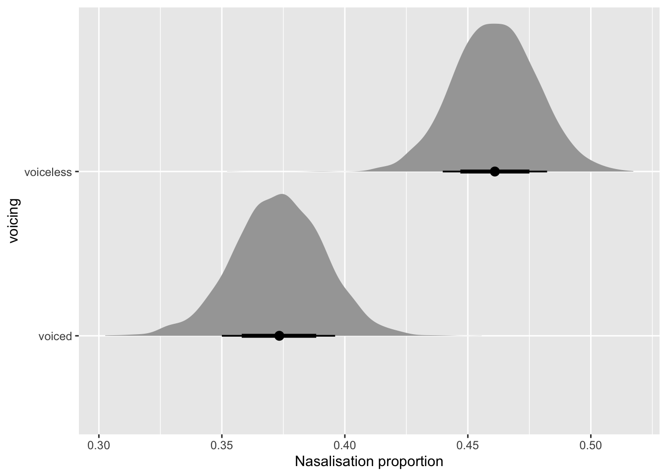
The plot suggests an overall greater nasalisation proportion in voiceless NC sequences. Let’s quantify how much greater it is, as we did in Section 4. We will use odds ratios in this context as well, i.e. we will convert log odds to odds ratios using the exp() (exponential) function (and as before we first calculate the difference and then exponentiate the resulting values, after which we can take summary measures, like means and quantile-based measures such as CrIs). Table 13 show the 90, 80 and 60% CrIs of the difference ratio of nasalisation proportion in voiceless vs voiced NC sequences.
nas_prop_bm_diff <- nas_prop_bm_draws_long_voicing |>
  # pivot data to create one column per voicing with the mean drawn values,
  # with one draw per raw. we need to drop the value_mean_prop col
  select(-value_mean_prop) |>
  pivot_wider(names_from = voicing, values_from = value_mean) |>
  mutate(
    # calculate the difference of voiceless and voiced in log odds
    voicing_diff = voicingvoiceless - voicingvoiced,
    # now transform with exp() to get the ratio difference
    voicing_diff_ratio = exp(voicing_diff)
  )

nas_prop_bm_diff_quant <- nas_prop_bm_diff |>
  reframe(
    # 90% CrI
    q90 = quantile2(voicing_diff_ratio, probs = c(0.05, 0.95)),
    # 80% CrI
    q80 = quantile2(voicing_diff_ratio, probs = c(0.1, 0.9)),
    # 60% CrI
    q60 = quantile2(voicing_diff_ratio, probs = c(0.2, 0.8)),
  ) |>
mutate(across(everything(), ~round(.x, 2)))| q90 | q80 | q60 |
|---|---|---|
| 1.23 | 1.27 | 1.33 |
| 1.69 | 1.63 | 1.56 |
The CrIs of the ratio difference in nasalisation proportion in voiceless vs voiced NC sequences suggest an increase of nasalisation in the voiceless NC sequences, with a 90% probability that the increase is between 23% and 69% of the proportion in voiced NC sequences.
Moving onto question 2: is there individual speaker variation? While in the recent tradition of linguistic research, varying (aka random) effects are used to control for differences across participants, it has been proposed to use the estimates of the varying coefficients to investigate individual differences (Tamminga et al., 2016). We will use the spread_draws() function from tidybayes (Kay, 2019) to extract the draws of the varying terms (in brms these are the coefficients that start with r_). There is quite a few steps of processing to get from the raw draws to the estimand we need: while we have commented the following code, we encourage readers to test each line sequentially and inspect the intermediate output to fully understand the process. We assume that readers are familiar enough with models with varying terms (aka random effects, mixed-effects, hierarchical, multilevel, nested models). What readers should note is that to obtain the expected predictions of nasalisation proportion for each speaker, the constant terms and the varying terms should be added (since the varying terms indicate the deviation of each speaker from the overall estimate).
library(tidybayes)

nas_prop_r <- nas_prop_bm |>
  # extract draws from model, only `r_speaker` varying terms
  spread_draws(r_speaker[speaker,voicingvowel]) |>
  # separate the column voicingvowel to two columns
  separate(voicingvowel, c("voicing", "vowel")) |>
  # join the draws with the `b_` terms
  left_join(y = nas_prop_bm_draws_long) |>
  # get the expected log-odd value of each speaker, in each draw
  # this is the sum of the `value` from the b_ terms and the value from the
  # r_speaker term.
  mutate(r_speaker_value = value + r_speaker) |>
  # group the data for summarise
  group_by(.draw, speaker, voicing) |>
  # get mean expected log odds by draw, speaker and voicing (averaging across vowel)
  summarise(r_speaker_value_mean = mean(r_speaker_value)) |>
  # make the data wider: two columns, one for voiced and one for voiceless
  pivot_wider(names_from = voicing, values_from = r_speaker_value_mean) |>
  # finally, calculate the difference in expected log odds of voiceless and voiced
  mutate(voicing_diff = voicingvoiceless - voicingvoiced)
Figure 12 plots the posterior distributions of the expected log-odd difference of coarticulatory nasalisation in voiceless vs voiced NC sequences (x-axis), for each speaker in the data (y-axis), as predicted by the model. The red solid vertical line indicates the constant (overall) expected log-odd difference based on the (constant) b_ terms. The black dashed vertical line marks log-difference 0 (i.e., no difference in proportion of nasalisation between voiceless and voiced NC).
nas_prop_r |>
  ggplot(aes(voicing_diff, reorder(speaker, voicing_diff))) +
  stat_halfeye() +
  geom_vline(xintercept = mean(nas_prop_bm_diff$voicing_diff), colour = "red") +
  geom_vline(xintercept = 0, linetype = "dashed") +
  lims(x = c(-1, 1.5)) +
  labs(
    x = "Log-odds difference between voiceless vs voiced NC sequences",
    y = "Speaker"
  )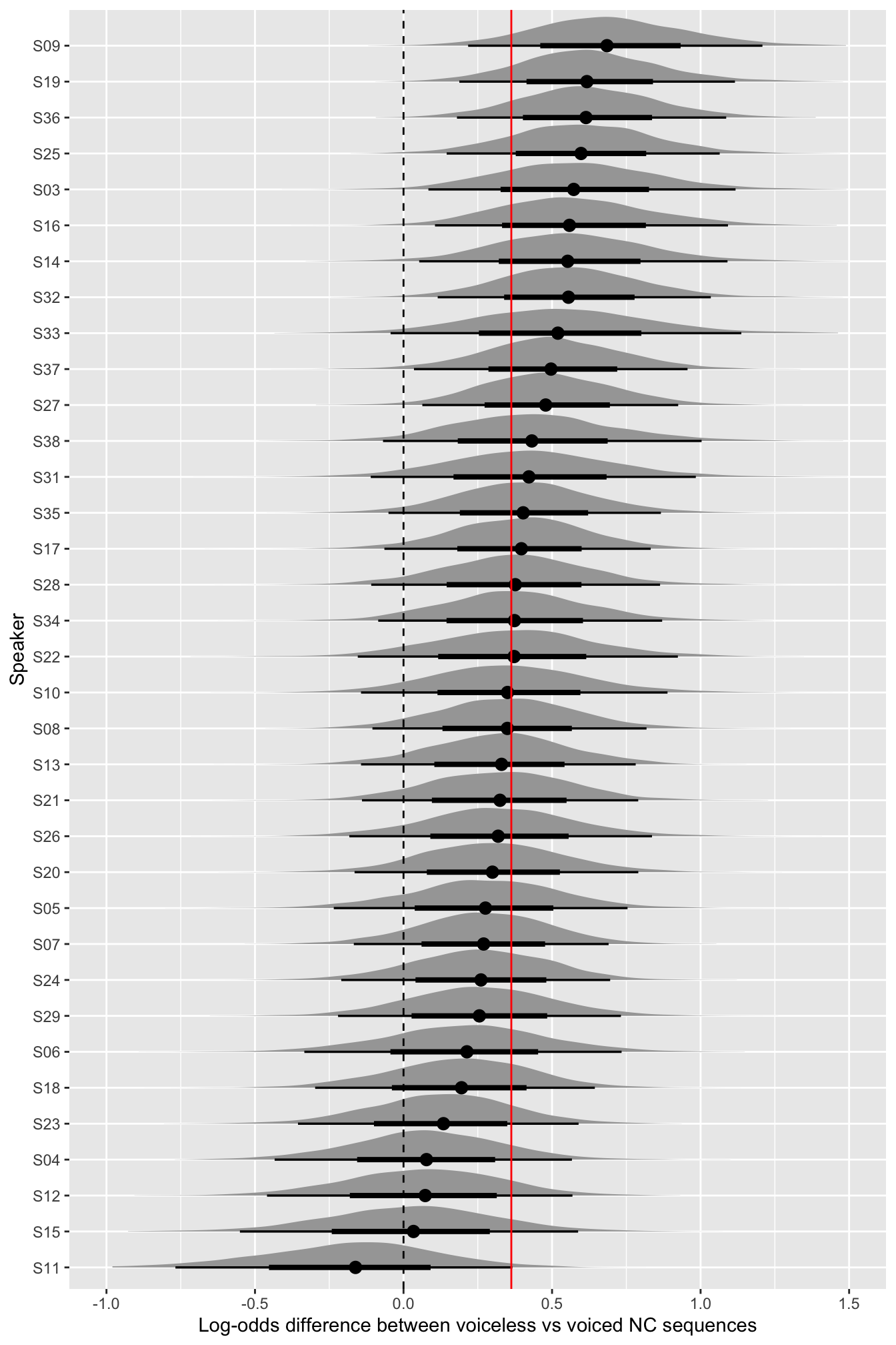
There is a lot of uncertainty within and between speakers: while the distributions of most speakers are located in the positive range, some expected distributions (see last 5 speakers at the bottom of figure) do substantially span both negative and positive values. In other words, while most speakers are more likely to have a larger nasalisation proportion in voiceless NC sequences, a few might in fact have the opposite pattern. Even among those speakers that do have a more robust positive difference, there is a lot of uncertainty as to the magnitude of the difference.
To conclude, previous work on coarticulatory nasalisation in English has suggested that vowels followed by an NC sequence where C is voiceless (NT) should show earlier coarticulatory nasalisation than vowels followed by an NC sequence where C is voiced (ND). We fitted a Bayesian beta regression model to assess this expectation. In sum, we find an increase of nasalisation proportion in the voiceless NC sequences compared to that of voiced NC sequences, with a 90% probability that the increase is between 23% and 69% of the proportion of voiced NC sequences. As for individual speakers’ variability, we find that while most speakers are more likely to have a larger nasalisation proportion in voiceless NC sequences, a few might have the opposite pattern.
Conclusion
In this tutorial we have presented two case studies where the outcome variable is a beta variable, i.e. a numeric continuous variable bounded between 0 and 1. We have shown how to fit Bayesian beta regressions to coarticulatory progressive voicing in voiceless stops in Italian in Section 4 and coarticulatory regressive nasalisation in vowels in German in Section 5. While this tutorial alone will not be sufficient to be able to independently run full Bayesian analyses, it will serve as a first introduction for readers to jump start their learning.
References
Abramson, A.S., Whalen, D.H., 2017. Voice onset time (VOT) at 50: Teoretical and practical issues in measuring voicing distinctions. Journal of Phonetics 63, 75–86. https://doi.org/10.1016/j.wocn.2017.05.002
Arel-Bundock, V., Greifer, N., Heiss, A., 2025. How to interpret statistical models using marginaleffects in R and Python. Journal of Statistical Software.
Arel-Bundock, V., Greifer, N., Heiss, A., 2024. How to interpret statistical models using marginaleffects for R and Python. Journal of Statistical Software 111, 1–32. https://doi.org/10.18637/jss.v111.i09
Baayen, R.H., 2008. Analyzing linguistic data: A practical introduction to statistics using R. Cambridge: Cambridge University Press. https://doi.org/10.1017/CBO9780511801686
Bates, D., Mächler, M., Bolker, B., Walker, S., 2015. Fitting linear mixed-effects models using lme4. Journal of Statistical Software 67, 1–48.
Beddor, P.S., 2009. A coarticulatory path to sound change. Language 785–821. https://doi.org/10.1353/lan.0.0165
Bockting, F., Radev, S.T., Bürkner, P.-C., 2024. Simulation-based prior knowledge elicitation for parametric Bayesian models. Scientific Reports 14, 17330. https://doi.org/10.1038/s41598-024-68090-7
Bonat, W.H., Jr, P.J.R., Zeviani, W.M., 2013. Regression models with responses on the unity Interval: Specification, estimation and comparison. Biometric Brazilian Journal 30, 18.
Bürkner, P.-C., 2021. Bayesian Item Response Modeling in R with brms and Stan. Journal of Statistical Software 100. https://doi.org/10.18637/jss.v100.i05
Bürkner, P.-C., 2018. Advanced Bayesian multilevel modeling with the R package brms. The R Journal 10, 395–411. https://doi.org/10.32614/RJ-2018-017
Bürkner, P.-C., 2017. Brms: An R package for Bayesian multilevel models using Stan. Journal of Statistical Software 80, 1–28. https://doi.org/10.18637/jss.v080.i01
Bürkner, P.C., 2025. The brms book: Applied Bayesian regression modelling using R and Stan.
Bürkner, P.C., Gabry, J., Kay, M., Vehtari, A., 2024. Posterior: Tools for working with posterior distributions.
Carignan, C., 2021. A practical method of estimating the time-varying degree of vowel nasalization from acoustic features. The Journal of the Acoustical Society of America 149, 911–922. https://doi.org/10.1121/10.0002925
Carignan, C., Shosted, R.K., Fu, M., Liang, Z.-P., Sutton, B.P., 2015. A real-time MRI investigation of the role of lingual and pharyngeal articulation in the production of the nasal vowel system of French. Journal of Phonetics 50, 34–51. https://doi.org/10.1016/j.wocn.2015.01.001
Cho, T., Kim, D., Kim, S., 2017. Prosodically-conditioned fine-tuning of coarticulatory vowel nasalization in English. Journal of Phonetics 64, 71–89. https://doi.org/10.1016/j.wocn.2016.12.003
Coretta, S., 2020. Vowel duration and consonant voicing: A production study (PhD thesis). The University of Manchester.
Coretta, S., 2019. Vowel duration, voicing duration, and vowel height: Acoustic and articulatory data from Italian [research compendium]. https://doi.org/10.17605/OSF.IO/XDGFZ
Coretta, S., Casillas, J.V., Roessig, S., Franke, M., Ahn, B., Al-Hoorie, A.H., Al-Tamimi, J., Alotaibi, N.E., AlShakhori, M.K., Altmiller, R.M., Arantes, P., Athanasopoulou, A., Baese-Berk, M.M., Bailey, G., Sangma, C.B.A., Beier, E.J., Benavides, G.M., Benker, N., BensonMeyer, E.P., Benway, N.R., Berry, G.M., Bing, L., Bjorndahl, C., Bolyanatz, M., Braver, A., Brown, V.A., Brown, A.M., Brugos, A., Buchanan, E.M., Butlin, T., Buxó-Lugo, A., Caillol, C., Cangemi, F., Carignan, C., Carraturo, S., Caudrelier, T., Chodroff, E., Cohn, M., Cronenberg, J., Crouzet, O., Dagar, E.L., Dawson, C., Diantoro, C.A., Dokovova, M., Drake, S., Du, F., Dubuis, M., Duême, F., Durward, M., Egurtzegi, A., Elsherif, M.M., Esser, J., Ferragne, E., Ferreira, F., Fink, L.K., Finley, S., Foster, K., Foulkes, P., Franzke, R., Frazer-McKee, G., Fromont, R., García, C., Geller, J., Grasso, C.L., Greca, P., Grice, M., Grose-Hodge, M.S., Gully, A.J., Halfacre, C., Hauser, I., Hay, J., Haywood, R., Hellmuth, S., Hilger, A.I., Holliday, N., Hoogland, D., Huang, Y., Hughes, V., Icardo Isasa, A., Ilchovska, Z.G., Jeon, H.-S., Jones, J., Junges, M.N., Kaefer, S., Kaland, C., Kelley, M.C., Kelly, N.E., Kettig, T., Khattab, G., Koolen, R., Krahmer, E., Krajewska, D., Krug, A., Kumar, A.A., Lander, A., Lentz, T.O., Li, W., Li, Y., Lialiou, M., Lima, R.M., Lo, J.J.H., Lopez Otero, J.C., Mackay, B., MacLeod, B., Mallard, M., McConnellogue, C.-A.M., Moroz, G., Murali, M., Nalborczyk, L., Nenadić, F., Nieder, J., Nikolić, D., Nogueira, F.G.S., Offerman, H.M., Passoni, E., Pélissier, M., Perry, S.J., Pfiffner, A.M., Proctor, M., Rhodes, R., Rodríguez, N., Roepke, E., Röer, J.P., Sbacco, L., Scarborough, R., Schaeffler, F., Schleef, E., Schmitz, D., Shiryaev, A., Sóskuthy, M., Spaniol, M., Stanley, J.A., Strickler, A., Tavano, A., Tomaschek, F., Tucker, B.V., Turnbull, R., Ugwuanyi, K.O., Urrestarazu-Porta, I., van de Vijver, R., Van Engen, K.J., van Miltenburg, E., Wang, B.X., Warner, N., Wehrle, S., Westerbeek, H., Wiener, S., Winters, S., Wong, S.G.-J., Wood, A., Wottawa, J., Xu, C., Zárate-Sández, G., Zellou, G., Zhang, C., Zhu, J., Roettger, T.B., 2023. Multidimensional Signals and Analytic Flexibility: Estimating Degrees of Freedom in Human-Speech Analyses. Advances in Methods and Practices in Psychological Science 6. https://doi.org/10.1177/25152459231162567
Cribari-Neto, F., Zeileis, A., 2010a. Beta Regression in r. Journal of Statistical Software 34. https://doi.org/10.18637/jss.v034.i02
Cribari-Neto, F., Zeileis, A., 2010b. Beta Regression in R. Journal of Statistical Software 34. https://doi.org/10.18637/jss.v034.i02
Davidson, L., 2016. Variability in the implementation of voicing in American English obstruents. Journal of Phonetics 54, 35–50. https://doi.org/10.1016/j.wocn.2015.09.003
Espinheira, P.L., Ferrari, S.L., Cribari-Neto, F., 2008. On beta regression residuals. Journal of Applied Statistics 35, 407–419.
Etz, A., Gronau, Q.F., Dablander, F., Edelsbrunner, P.A., Baribault, B., 2018. How to become a Bayesian in eight easy steps: An annotated reading list. Psychonomic Bulletin & Review 25, 219–234. https://doi.org/10.3758/s13423-017-1317-5
Ferrari, S., Cribari-Neto, F., 2004. Beta Regression for Modelling Rates and Proportions. Journal of Applied Statistics 31, 799–815. https://doi.org/10.1080/0266476042000214501
Fowler, C.A., 2005. Parsing coarticulated speech in perception: Effects of coarticulation resistance. Journal of Phonetics 33, 199–213. https://doi.org/10.1016/j.wocn.2004.10.003
Gelman, A., 2005. Analysis of variance—why it is more important than ever. The Annals of Statistics 33. https://doi.org/10.1214/009053604000001048
Gelman, A., Hill, J., Yajima, M., 2012. Why We (Usually) Don’t Have to Worry About Multiple Comparisons. Journal of Research on Educational Effectiveness 5, 189–211. https://doi.org/10.1080/19345747.2011.618213
Gick, B., Wilson, I., Derrick, D., 2013. Articulatory phonetics. Wiley-Blackwell.
Gupta, A.K., Nadarajah, S., 2014. Handbook of Beta Distribution and Its Applications. CRC Press, Boca Raton. https://doi.org/10.1201/9781482276596
Heiss, A., 2021. A guide to modeling proportions with Bayesian beta and zero-inflated beta regression models.
Herbst, C.T., Schutte, H.K., Bowling, D.L., Svec, J.G., 2017. Comparing chalk with cheese: The EGG contact quotient is only a limited surrogate of the closed quotient. Journal of Voice 31, 401–409. https://doi.org/10.1016/j.jvoice.2016.11.007
Johnson, K., 2003. Acoustic and auditory phonetics. Wiley-Blackwell. https://doi.org/10.1159/000078663
Kay, M., 2023. Ggdist: Visualizations of Distributions and Uncertainty in the Grammar of Graphics. IEEE Transactions on Visualization and Computer Graphics 1–11. https://doi.org/10.1109/TVCG.2023.3327195
Kay, M., 2019. Tidybayes: Tidy data and geoms for Bayesian models.
Kieschnick, R., McCullough, B.D., 2003. Regression analysis of variates observed on (0, 1): Percentages, proportions and fractions. Statistical Modelling 3, 193–213. https://doi.org/10.1191/1471082X03st053oa
Kirby, J., Sonderegger, M., 2018. Mixed-effects design analysis for experimental phonetics. Journal of Phonetics 70, 70–85. https://doi.org/10.1016/j.wocn.2018.05.005
Kluender, K.R., Diehl, R.L., Wright, B.A., 1988. Vowel-length differences before voiced and voiceless consonants: An auditory explanation. Journal of Phonetics 16, 153–169. https://doi.org/10.1016/S0095-4470(19)30480-2
Kosmidis, I., Zeileis, A., 2024. Extended-support beta regression for [0, 1] responses. https://doi.org/10.48550/ARXIV.2409.07233
Krysicki, W., 1999. On some new properties of the beta distribution. Statistics & Probability Letters 42, 131–137. https://doi.org/10.1016/S0167-7152(98)00197-7
Ladefoged, P., Johnson, K., 2014. A course in phonetics. Cengage learning.
López, F.O., 2013. A Bayesian Approach to Parameter Estimation in Simplex Regression Model: A Comparison with Beta Regression. Revista Colombiana de Estadística 21.
McElreath, R., 2020. Statistical rethinking: a Bayesian course with examples in R and Stan, Second edition. ed, Chapman & Hall/CRC texts in statistical science series. CRC Press, Boca Raton.
McElreath, R., 2019. Statistical rethinking: A Bayesian course with examples in R and Stan. Boca Raton, FL: CRC Press.
Mikkola, P., Martin, O.A., Chandramouli, S., Hartmann, M., Abril Pla, O., Thomas, O., Pesonen, H., Corander, J., Vehtari, A., Kaski, S., Bürkner, P.-C., Klami, A., 2024. Prior knowledge elicitation: The past, present, and future. Bayesian Analysis 19. https://doi.org/10.1214/23-BA1381
Nalborczyk, L., Batailler, C., Loevenbruck, H., Vilain, A., Bürkner, P.-C., 2019. An introduction to bayesian multilevel models using brms: A case study of gender effects on vowel variability in standard indonesian. Journal of Speech, Language, and Hearing Research. https://doi.org/10.1044/2018_JSLHR-S-18-0006
Ohala, J.J., 2011. Accommodation to the aerodynamic voicing constraint and its phonological relevance, in: Proceedings of the 17th International Congress of Phonetic Sciences. pp. 64–67.
Politzer-Ahles, S., Piccinini, P., 2018. On visualizing phonetic data from repeated measures experiments with multiple random effects. Journal of Phonetics. https://doi.org/10.1016/j.wocn.2018.05.002
Roettger, T.B., Winter, B., Baayen, H., 2018. Emergent data analysis in phonetic sciences: Towards pluralism and reproducibility. Journal of Phonetics 73, 1–7. https://doi.org/10.1016/j.wocn.2018.12.001
Rosen, K.M., 2005. Analysis of speech segment duration with the lognormal distribution: A basis for unification and comparison. Journal of Phonetics 33, 411–426. https://doi.org/10.1016/j.wocn.2005.02.001
Rothenberg, M., 1967. The breath-stream dynamics of simple-released-plosive production. Basel: Biblioteca Phonetica.
Scholz, M., Bürkner, P.-C., 2025. Prediction can be safely used as a proxy for explanation in causally consistent bayesian generalized linear models. Journal of Statistical Computation and Simulation 1–24.
Scholz, M., Bürkner, P.-C., 2023. Posterior accuracy and calibration under misspecification in bayesian generalized linear models. arXiv preprint arXiv:2311.09081.
Stan Development Team, 2025. Prior Choice Recommendations.
Stan Development Team, 2017. Stan: A C++ library for probability and sampling, version 2.14.0.
Tamminga, M., Ahern, C., Ecay, A., 2016. Generalized additive mixed models for intraspeaker variation. Linguistics Vanguard 2, 33–41. https://doi.org/10.1515/lingvan-2016-0030
Tavakoli, S., Matteo, B., Pigoli, D., Chodroff, E., Coleman, J., Gubian, M., Renwick, M.E.L., Sonderegger, M., 2024. Statistics in phonetics. Annual Review of Statistics and Its Application. https://doi.org/10.1146/annurev-statistics-112723-034642
van den Berg, J., 1958. Myoelastic-aerodynamic theory of voice production. Journal of Speech and Hearing Research 1, 227–244. https://doi.org/10.1044/jshr.0103.227
Vasishth, S., Beckman, M., Nicenboim, B., Li, F., Kong, E.J., 2018. Bayesian data analysis in the phonetic sciences: A tutorial introduction. Journal of Phonetics 71, 147–161. https://doi.org/10.1016/j.wocn.2018.07.008
Verissimo, J., 2021. Analysis of rating scales: A pervasive problem in bilingualism research and a solution with Bayesian ordinal models. Bilingualism: Language and Cognition 24, 842–848. https://doi.org/10.1017/S1366728921000316
Wickham, H., Averick, M., Bryan, J., Chang, W., McGowan, L., François, R., Grolemund, G., Hayes, A., Henry, L., Hester, J., Kuhn, M., Pedersen, T., Miller, E., Bache, S., Müller, K., Ooms, J., Robinson, D., Seidel, D., Spinu, V., Takahashi, K., Vaughan, D., Wilke, C., Woo, K., Yutani, H., 2019. Welcome to the Tidyverse. Journal of Open Source Software 4, 1686. https://doi.org/10.21105/joss.01686
Winter, B., 2020. Statistics for Linguists: An Introduction Using R. Routledge.
Footnotes
The \(\mu\), \(\phi\) parametrisation is equivalent to the \(\alpha\), \(\beta\) parametrisation in that \(\alpha = \mu\phi\) and \(\beta = (1-\mu)\phi\). Using the former allows brms to exploit the same programmatic features of other distributions parametrised with a location parameter.↩︎
While the terms “random effects, intercept and slopes” are commonly employed in applied statistical work in linguistics and phonetics, we opt to use the conceptually more appropriate terminology proposed by (Gelman, 2005): varying terms, intercepts, slopes, coefficients. Other common terms are multilevel and hierarchical terms. Note that with “varying terms” we refer specifically to model terms with partial pooling in opposition to “constant terms” estimated with no pooling (McElreath, 2020, p. 408). See (Nalborczyk et al., 2019) for a detailed overview.↩︎
For a discussion on multiple comparisons in Bayesian statistics, see (Gelman et al., 2012). If multiple comparisons fixed effects is performed and one worries about their joint frequentist error rates, one could, for example, increase the width of the credible intervals for more conservative inference.↩︎