Analysis of intrinsic vowel duration in Northwestern Italian

1 Attach packages

library(tidyverse)
theme_set(theme_light())
library(magrittr)
library(coretta2018itaegg)
library(brms)
library(rstan)
library(posterior)
library(tidybayes)
library(ggdist)
library(mgcv)
library(tidygam)
library(HDInterval)
library(truncdist)
library(ggdist)

my_seed <- 9899

cols <- viridisLite::viridis(5)
cols[5] <- "#d95f02"

2 Read data

The following code loads the data from the coretta2018itaegg package and creates new variables as transformations of the existing ones.

data("ita_egg")

ita_egg <- ita_egg |> 
  drop_na(f13, f23) |> 
  mutate(
  duration = v1_duration,
  vowel = as.factor(vowel),
  c1_place = as.factor(c1_place),
  c2_place = as.factor(c2_place),
  duration_z = as.vector(scale(duration)),
  duration_log = log(duration),
  duration_logz = as.vector(scale(log(duration))),
  speech_rate_log = log(speech_rate),
  speech_rate_logz = as.vector(scale(log(speech_rate_log))),
  f13_z = as.vector(scale(f13)),
  f23_z = as.vector(scale(f23)),
  speaker = as.factor(speaker),
  word_ipa = str_replace_all(word, "ch|c", "k"),
  previous_sound = str_sub(word_ipa, 1, 1),
  next_sound = str_sub(word_ipa, 3, 3)
)

3 Plotting

ita_egg |>
  group_by(speaker) |>
  mutate(
    f13_speaker_z = as.vector(scale(f13)),
    f23_speaker_z = as.vector(scale(f23))
  ) |>
  ggplot(aes(f23_speaker_z, f13_speaker_z, colour = vowel)) +
  geom_point(alpha = 0.2) +
  stat_ellipse(type = "norm") +
  scale_x_reverse(position = "top") + scale_y_reverse(position = "right") +
  coord_fixed()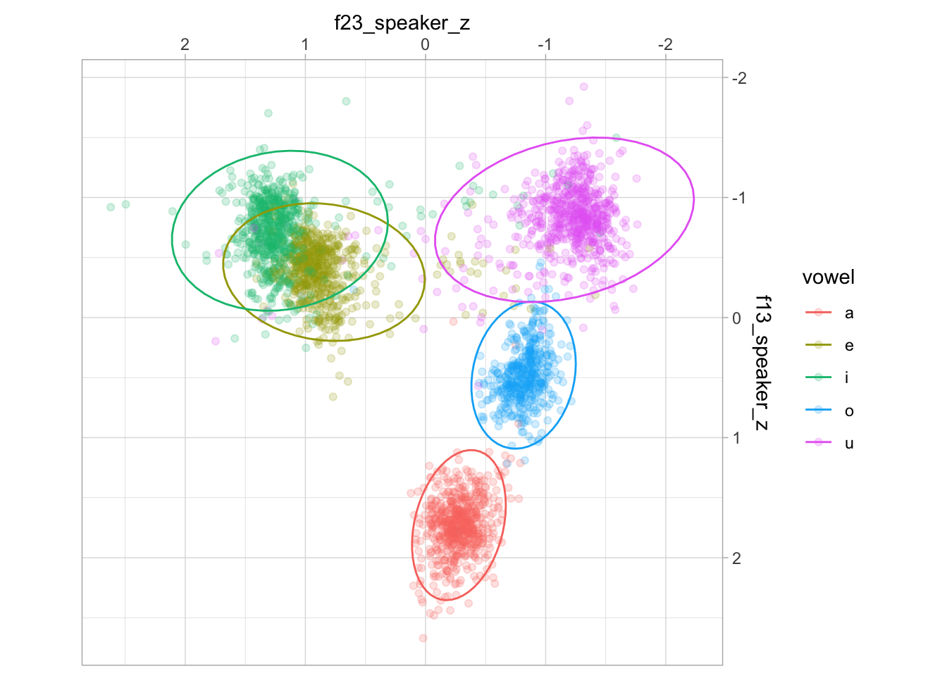

ita_egg |>
  group_by(speaker) |>
  mutate(
    f13_speaker_z = as.vector(scale(f13)),
    f23_speaker_z = as.vector(scale(f23))
  ) |>
  ggplot(aes(f23_speaker_z, f13_speaker_z)) +
  geom_point(aes(colour = duration), alpha = 0.8) +
  stat_ellipse(aes(group = vowel), type = "norm") +
  scale_x_reverse(position = "top") + scale_y_reverse(position = "right") +
  coord_fixed()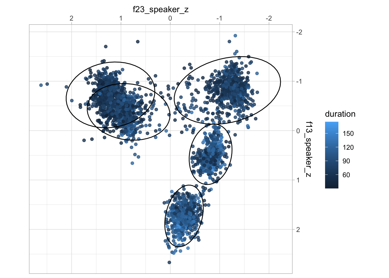

ita_egg |>
  ggplot(aes(f13_z, duration_z)) +
  geom_density_2d_filled()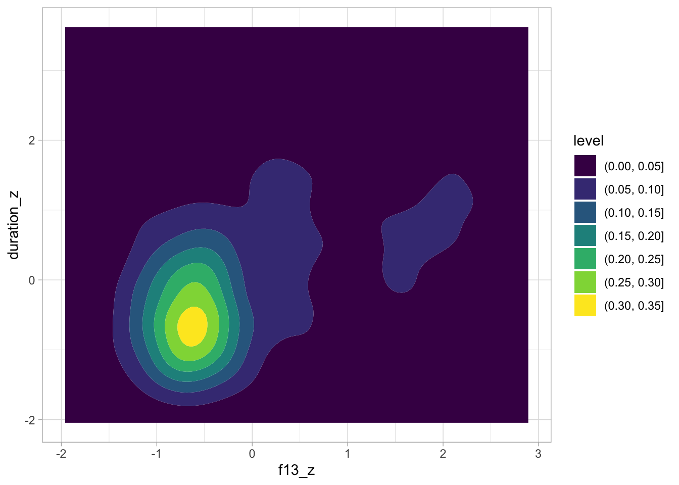

ita_egg |> 
  ggplot(aes(vowel, duration)) +
  geom_jitter(width = 0.2, alpha = 0.2) +
  facet_grid(rows = vars(next_sound), cols = vars(previous_sound))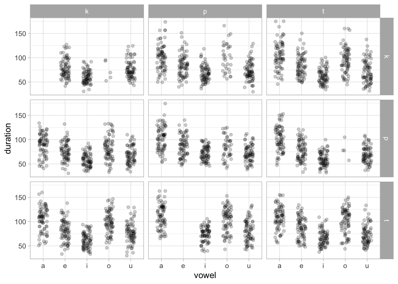

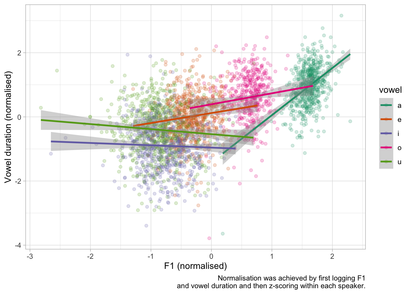
ita_egg |> 
  group_by(speaker) |>
  mutate(
    f13_speaker_z = as.vector(scale(log(f13))),
    duration_speaker_z = as.vector(scale(log(duration)))
  ) |>
  ggplot(aes(f13_speaker_z, duration_speaker_z, colour = vowel)) +
  geom_point(alpha = 0.2) +
  geom_smooth(method = "lm", formula = y ~ x) +
  scale_color_brewer(type = "qual", palette = "Dark2") +
  labs(
    x = "F1 (normalised)",
    y = "Vowel duration (normalised)",
    caption = "Normalisation was achieved by first logging F1\nand vowel duration and then z-scoring within each speaker."
  )

ggsave("img/dur-f1.png", width = 7, height = 5)

4 Linear modelling

4.1 Prior predictive checks

The outcome duration_logz and predictor f13_z are z-scored and the intercept has been suppressed so that the indexing method is used for the vowel predictor instead of contrasts.

The following code sets up the model formula and gets the default priors. This is the mathematical representation of the model.

$$ \[\begin{align*} y_i &\sim \mathcal{N}(\mu_i, \sigma) \\ \mu_i &= a_i + b_i \cdot \text{F1}_i + c_i \cdot sr_i \\ a_i &= \alpha_{\text{vowel}[i], \,\text{c1}[i], \,\text{c2}[i]} + u^{(a)}_{\text{speaker}[i], \,\text{vowel}[i], \,\text{c1}[i], \,\text{c2}[i]} \\ b_i &= \beta_{\text{vowel}[i], \,\text{c1}[i], \,\text{c2}[i]} + u^{(b)}_{\text{speaker}[i], \,\text{vowel}[i], \,\text{c1}[i], \,\text{c2}[i]} \\ c_i &= \gamma + u^{(c)}_{\text{speaker}[i]} \\ \begin{bmatrix} u^{(a)}_{\text{speaker}[i], \cdot} \\ u^{(b)}_{\text{speaker}[i], \cdot} \end{bmatrix} &\sim \mathcal{N}\!\left( \mathbf{0}, \, \Sigma \right), \quad u^{(c)}_{\text{speaker}[i]} \sim \mathcal{N}(0, \tau_c^2) \end{align*}\]

$$

The \(a_i\) and \(b_i\) coefficients correspond to the by-vowel intercept and the F1 effect.

bm_1_f <- bf(
  duration_logz ~ a + b*f13_z + c*speech_rate_logz,
  a ~ 0 + vowel:c1_place:c2_place + (0 + vowel:c1_place:c2_place | speaker),
  b ~ 0 + vowel:c1_place:c2_place + (0 + vowel:c1_place:c2_place | speaker),
  c ~ (1 | speaker),
  nl = TRUE
)

bm_1_get <- get_prior(
  bm_1_f,
  data = ita_egg,
  family = gaussian,
) |> as_tibble()
bm_1_get

# A tibble: 194 × 10
   prior                  class coef  group resp  dpar  nlpar lb    ub    source
   <chr>                  <chr> <chr> <chr> <chr> <chr> <chr> <chr> <chr> <chr> 
 1 "lkj(1)"               cor   ""    ""    ""    ""    ""    ""    ""    defau…
 2 ""                     cor   ""    "spe… ""    ""    ""    ""    ""    defau…
 3 "student_t(3, 0, 2.5)" sigma ""    ""    ""    ""    ""    "0"   ""    defau…
 4 ""                     b     ""    ""    ""    ""    "a"   ""    ""    defau…
 5 ""                     b     "vow… ""    ""    ""    "a"   ""    ""    defau…
 6 ""                     b     "vow… ""    ""    ""    "a"   ""    ""    defau…
 7 ""                     b     "vow… ""    ""    ""    "a"   ""    ""    defau…
 8 ""                     b     "vow… ""    ""    ""    "a"   ""    ""    defau…
 9 ""                     b     "vow… ""    ""    ""    "a"   ""    ""    defau…
10 ""                     b     "vow… ""    ""    ""    "a"   ""    ""    defau…
# ℹ 184 more rows

We fit the prior predictive model with relatively weakly informative priors. The prior predictive model is the model fitted with sample_prior = "only" so that only the priors are sampled, without including the data. This enables us to check the joint predictions based on priors only.

priors <- c(
  prior(normal(0, 1), class = b, nlpar = a),
  prior(normal(0, 1), class = b, nlpar = b),
  prior(normal(0, 0.1), class = b, nlpar = c),
  prior(cauchy(0, 0.1), class = sigma),
  prior(lkj(2), class = cor),
  prior(cauchy(0, 0.1), class = sd, nlpar = a),
  prior(cauchy(0, 0.1), class = sd, nlpar = b),
  prior(cauchy(0, 0.1), class = sd, nlpar = c)
)


bm_1_priors <- brm(
  bm_1_f,
  family = gaussian,
  data = ita_egg,
  prior = priors,
  cores = 4,
  init = 0,
  threads = threading(2),
  backend = "cmdstanr",
  sample_prior = "only",
  file = "data/cache/bm_1_priors",
)

The following plots show the prior predictive values of vowel duration, based exclusively on the priors. The prior predictive plots indicate that the priors cover a reasonable range of values without being too informative.

conditional_effects(bm_1_priors, "f13_z:vowel", spaghetti = TRUE, ndraws = 50)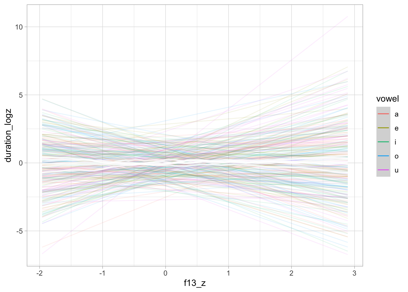

conditional_effects(bm_1_priors, "f13_z:c1_place", spaghetti = TRUE, ndraws = 50)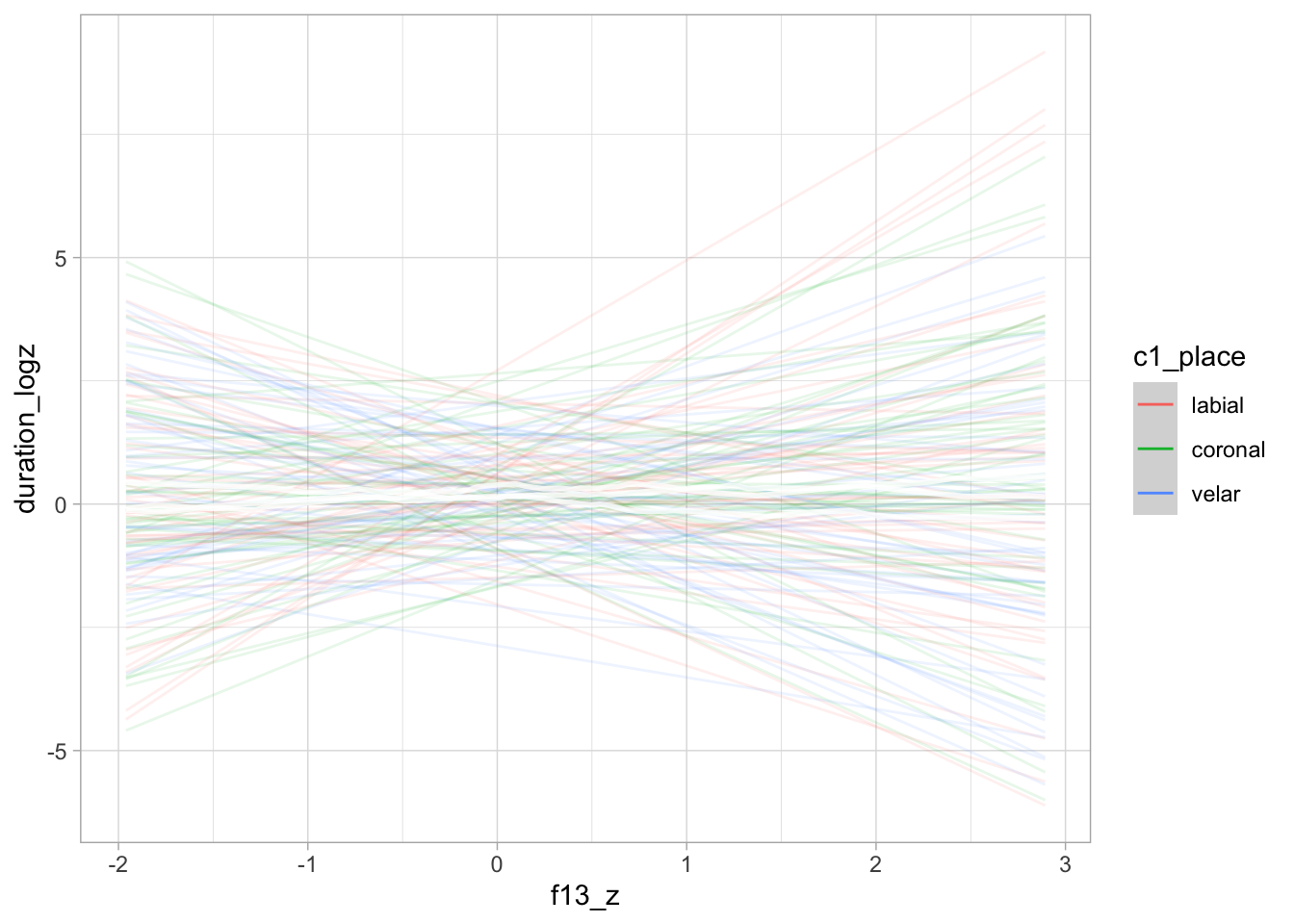

conditional_effects(bm_1_priors, "f13_z:c2_place", spaghetti = TRUE, ndraws = 50)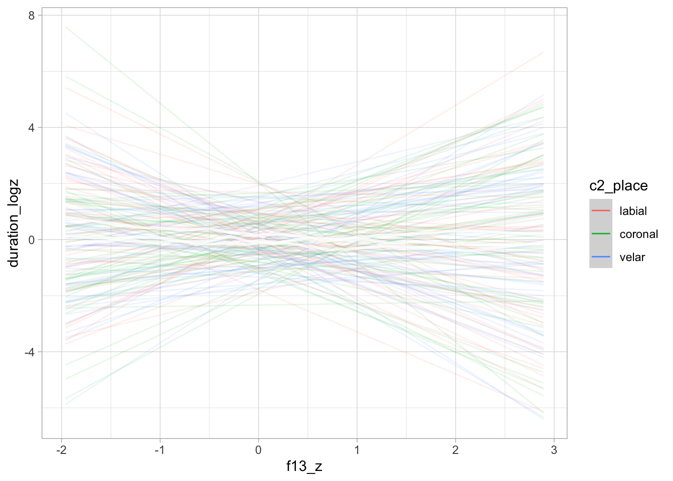

conditional_effects(bm_1_priors, "speech_rate_logz", spaghetti = TRUE, ndraws = 50)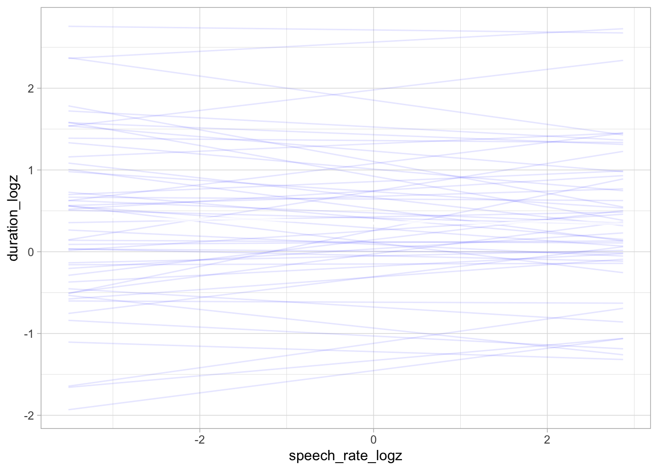

conditional_effects(bm_1_priors, "vowel")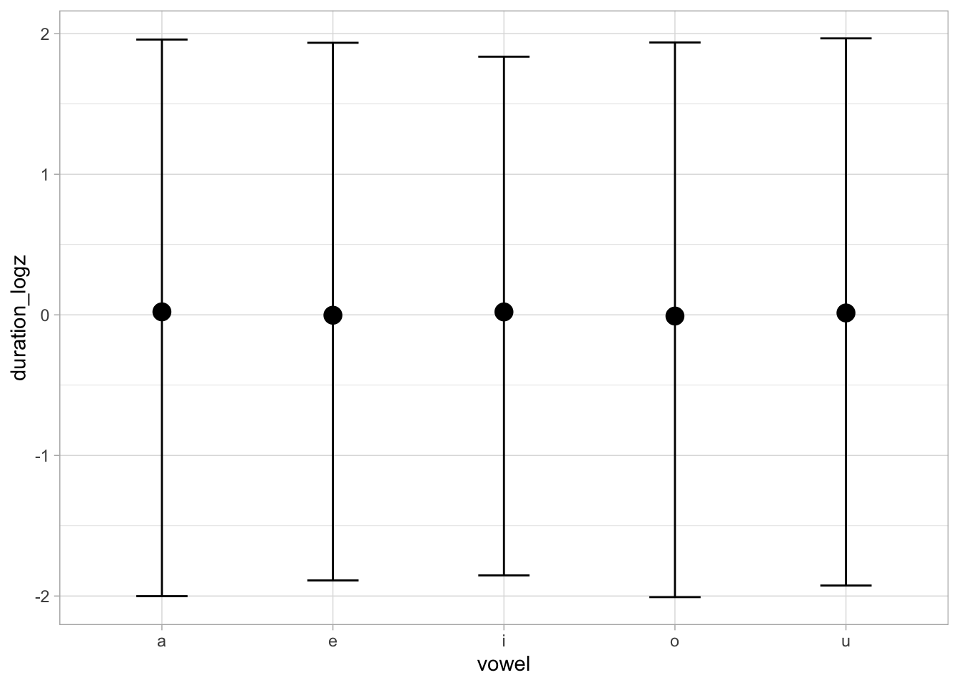

4.2 Model fit

We now fit the model with the specified priors to the data.

bm_1 <- brm(
  bm_1_f,
  family = gaussian,
  data = ita_egg,
  prior = priors,
  init = 0,
  cores = 4,
  threads = threading(2),
  backend = "cmdstanr",
  file = "data/cache/bm_1",
)

The following are the regression coefficients as estimated by the model.

fixef(bm_1, probs = c(0.05, 0.95)) |> round(2)

                                         Estimate Est.Error    Q5   Q95
a_vowela:c1_placelabial:c2_placelabial      -0.05      0.29 -0.55  0.42
a_vowele:c1_placelabial:c2_placelabial       0.38      0.13  0.17  0.59
a_voweli:c1_placelabial:c2_placelabial      -0.31      0.13 -0.54 -0.09
a_vowelo:c1_placelabial:c2_placelabial       0.10      0.19 -0.21  0.41
a_vowelu:c1_placelabial:c2_placelabial      -0.48      0.18 -0.77 -0.17
a_vowela:c1_placecoronal:c2_placelabial     -0.12      0.26 -0.56  0.30
a_vowele:c1_placecoronal:c2_placelabial      0.10      0.15 -0.14  0.34
a_voweli:c1_placecoronal:c2_placelabial     -0.89      0.18 -1.18 -0.61
a_vowelo:c1_placecoronal:c2_placelabial      0.19      0.29 -0.26  0.67
a_vowelu:c1_placecoronal:c2_placelabial     -0.55      0.18 -0.84 -0.25
a_vowela:c1_placevelar:c2_placelabial       -0.22      0.27 -0.69  0.22
a_vowele:c1_placevelar:c2_placelabial       -0.03      0.13 -0.23  0.19
a_voweli:c1_placevelar:c2_placelabial       -1.15      0.16 -1.41 -0.89
a_vowelo:c1_placevelar:c2_placelabial       -0.07      0.14 -0.30  0.15
a_vowelu:c1_placevelar:c2_placelabial       -0.46      0.23 -0.84 -0.08
a_vowela:c1_placelabial:c2_placecoronal      0.20      0.29 -0.29  0.68
a_vowele:c1_placelabial:c2_placecoronal      0.00      1.00 -1.65  1.65
a_voweli:c1_placelabial:c2_placecoronal     -0.33      0.15 -0.57 -0.08
a_vowelo:c1_placelabial:c2_placecoronal      0.53      0.17  0.25  0.80
a_vowelu:c1_placelabial:c2_placecoronal     -0.20      0.18 -0.50  0.10
a_vowela:c1_placecoronal:c2_placecoronal     0.38      0.30 -0.12  0.87
a_vowele:c1_placecoronal:c2_placecoronal     0.40      0.14  0.18  0.62
a_voweli:c1_placecoronal:c2_placecoronal    -0.53      0.18 -0.83 -0.24
a_vowelo:c1_placecoronal:c2_placecoronal     0.38      0.16  0.13  0.64
a_vowelu:c1_placecoronal:c2_placecoronal    -0.30      0.21 -0.64  0.04
a_vowela:c1_placevelar:c2_placecoronal       0.17      0.30 -0.33  0.65
a_vowele:c1_placevelar:c2_placecoronal       0.14      0.13 -0.07  0.36
a_voweli:c1_placevelar:c2_placecoronal      -0.56      0.18 -0.85 -0.25
a_vowelo:c1_placevelar:c2_placecoronal       0.69      0.14  0.45  0.93
a_vowelu:c1_placevelar:c2_placecoronal       0.00      0.20 -0.33  0.32
a_vowela:c1_placelabial:c2_placevelar        0.34      0.33 -0.21  0.88
a_vowele:c1_placelabial:c2_placevelar        0.18      0.11  0.01  0.35
a_voweli:c1_placelabial:c2_placevelar       -0.44      0.15 -0.69 -0.19
a_vowelo:c1_placelabial:c2_placevelar        0.55      0.20  0.21  0.87
a_vowelu:c1_placelabial:c2_placevelar        0.08      0.21 -0.25  0.43
a_vowela:c1_placecoronal:c2_placevelar       0.31      0.29 -0.18  0.78
a_vowele:c1_placecoronal:c2_placevelar       0.33      0.12  0.13  0.52
a_voweli:c1_placecoronal:c2_placevelar      -0.74      0.16 -0.99 -0.48
a_vowelo:c1_placecoronal:c2_placevelar       0.43      0.15  0.18  0.67
a_vowelu:c1_placecoronal:c2_placevelar      -0.58      0.20 -0.91 -0.25
a_vowela:c1_placevelar:c2_placevelar         0.01      1.02 -1.66  1.66
a_vowele:c1_placevelar:c2_placevelar         0.10      0.12 -0.10  0.30
a_voweli:c1_placevelar:c2_placevelar        -0.88      0.14 -1.11 -0.65
a_vowelo:c1_placevelar:c2_placevelar        -0.22      0.27 -0.64  0.21
a_vowelu:c1_placevelar:c2_placevelar        -0.30      0.19 -0.60  0.02
b_vowela:c1_placelabial:c2_placelabial       0.49      0.17  0.22  0.77
b_vowele:c1_placelabial:c2_placelabial       0.46      0.25  0.05  0.89
b_voweli:c1_placelabial:c2_placelabial       0.05      0.17 -0.24  0.33
b_vowelo:c1_placelabial:c2_placelabial       0.17      0.36 -0.43  0.76
b_vowelu:c1_placelabial:c2_placelabial      -0.16      0.21 -0.50  0.19
b_vowela:c1_placecoronal:c2_placelabial      0.50      0.15  0.27  0.75
b_vowele:c1_placecoronal:c2_placelabial      0.58      0.28  0.13  1.03
b_voweli:c1_placecoronal:c2_placelabial      0.03      0.22 -0.33  0.37
b_vowelo:c1_placecoronal:c2_placelabial      0.30      0.58 -0.66  1.20
b_vowelu:c1_placecoronal:c2_placelabial     -0.11      0.19 -0.43  0.20
b_vowela:c1_placevelar:c2_placelabial        0.37      0.16  0.11  0.64
b_vowele:c1_placevelar:c2_placelabial        0.51      0.24  0.11  0.91
b_voweli:c1_placevelar:c2_placelabial       -0.17      0.20 -0.50  0.16
b_vowelo:c1_placevelar:c2_placelabial        0.26      0.22 -0.09  0.62
b_vowelu:c1_placevelar:c2_placelabial        0.03      0.26 -0.39  0.47
b_vowela:c1_placelabial:c2_placecoronal      0.48      0.16  0.22  0.76
b_vowele:c1_placelabial:c2_placecoronal      0.00      0.99 -1.61  1.61
b_voweli:c1_placelabial:c2_placecoronal     -0.12      0.20 -0.45  0.21
b_vowelo:c1_placelabial:c2_placecoronal      0.52      0.30  0.03  1.01
b_vowelu:c1_placelabial:c2_placecoronal     -0.23      0.21 -0.58  0.11
b_vowela:c1_placecoronal:c2_placecoronal     0.35      0.17  0.07  0.63
b_vowele:c1_placecoronal:c2_placecoronal     0.42      0.25  0.01  0.83
b_voweli:c1_placecoronal:c2_placecoronal     0.08      0.21 -0.26  0.44
b_vowelo:c1_placecoronal:c2_placecoronal     0.73      0.24  0.33  1.12
b_vowelu:c1_placecoronal:c2_placecoronal     0.02      0.22 -0.33  0.37
b_vowela:c1_placevelar:c2_placecoronal       0.40      0.17  0.12  0.68
b_vowele:c1_placevelar:c2_placecoronal       0.40      0.24  0.01  0.80
b_voweli:c1_placevelar:c2_placecoronal       0.39      0.22  0.04  0.75
b_vowelo:c1_placevelar:c2_placecoronal      -0.15      0.24 -0.55  0.25
b_vowelu:c1_placevelar:c2_placecoronal       0.23      0.21 -0.13  0.57
b_vowela:c1_placelabial:c2_placevelar        0.22      0.19 -0.09  0.55
b_vowele:c1_placelabial:c2_placevelar        0.22      0.21 -0.12  0.56
b_voweli:c1_placelabial:c2_placevelar        0.10      0.19 -0.21  0.41
b_vowelo:c1_placelabial:c2_placevelar       -0.06      0.31 -0.57  0.46
b_vowelu:c1_placelabial:c2_placevelar        0.56      0.24  0.18  0.94
b_vowela:c1_placecoronal:c2_placevelar       0.30      0.16  0.04  0.57
b_vowele:c1_placecoronal:c2_placevelar       0.76      0.24  0.36  1.16
b_voweli:c1_placecoronal:c2_placevelar       0.13      0.21 -0.21  0.47
b_vowelo:c1_placecoronal:c2_placevelar       0.18      0.23 -0.21  0.55
b_vowelu:c1_placecoronal:c2_placevelar      -0.21      0.22 -0.57  0.14
b_vowela:c1_placevelar:c2_placevelar        -0.01      1.00 -1.66  1.65
b_vowele:c1_placevelar:c2_placevelar         0.57      0.23  0.19  0.96
b_voweli:c1_placevelar:c2_placevelar         0.04      0.19 -0.26  0.35
b_vowelo:c1_placevelar:c2_placevelar         1.12      0.63  0.02  2.10
b_vowelu:c1_placevelar:c2_placevelar        -0.13      0.21 -0.47  0.22
c_Intercept                                 -0.29      0.03 -0.34 -0.23

We can now extract the MCMC draws of the \(\alpha\) and \(\beta\) coefficients for further processing. We convert the draws to a long format.

bm_1_draws <- as_draws_df(bm_1)

bm_1_draws_long <- bm_1_draws |> 
  select(
    `b_a_vowela:c1_placelabial:c2_placelabial`:`b_b_vowelu:c1_placevelar:c2_placevelar`,
    .chain, .iteration, .draw
  ) |> 
  pivot_longer(
    `b_a_vowela:c1_placelabial:c2_placelabial`:`b_b_vowelu:c1_placevelar:c2_placevelar`
    ) |> 
  separate(name, c("vowel", "c1_place", "c2_place"), sep = ":") |> 
  separate(vowel, c("par", "coef", "vowel"))

The following code summarises the draws for each coefficients, by vowel but averaged across the consonant place of articulation. a is the by-vowel intercept, while b is the effect of F1.

bm_1_draws_long_avg <- bm_1_draws_long |> 
  group_by(.chain, .iteration, .draw, coef, vowel) |> 
  summarise(epred = mean(value), .groups = "drop") |> 
  mutate(
    vowel = str_remove(vowel, "vowel")
  )

bm_1_draws_long_avg |> 
  group_by(coef, vowel) |> 
  summarise(
    mean = mean(epred),
    lo_90 = quantile2(epred, 0.05),
    hi_90 = quantile2(epred, 0.95),
    .groups = "drop"
  ) |> 
  mutate(across(where(is.numeric), ~round(., 2)))

# A tibble: 10 × 5
   coef  vowel  mean lo_90 hi_90
   <chr> <chr> <dbl> <dbl> <dbl>
 1 a     a      0.11 -0.14  0.36
 2 a     e      0.18 -0.02  0.37
 3 a     i     -0.65 -0.74 -0.55
 4 a     o      0.29  0.17  0.4 
 5 a     u     -0.31 -0.44 -0.19
 6 b     a      0.35  0.14  0.56
 7 b     e      0.44  0.22  0.66
 8 b     i      0.06 -0.06  0.17
 9 b     o      0.34  0.14  0.54
10 b     u      0    -0.13  0.12

4.3 Coefficient b

This section focusses on the coefficient b, the effect of F1, by vowel and place of articulation.

bm_1_draws_long_avg_pl_vow <- bm_1_draws_long |> 
  group_by(.chain, .iteration, .draw, coef, vowel, c1_place, c2_place) |> 
  summarise(epred = mean(value), .groups = "drop") |> 
  mutate(
    c1_place = str_remove(c1_place, "c1_place") |> str_sub(1, 3),
    c2_place = str_remove(c2_place, "c2_place") |> str_sub(1, 3),
    vowel = str_remove(vowel, "vowel")
  ) |> 
  unite("c1_c2", c1_place, c2_place)

bm_1_draws_long_avg_pl_vow |> 
  filter(coef == "b") |> 
  group_by(c1_c2, vowel) |> 
  summarise(
    mean = mean(epred), sd = sd(epred),
    lo_90 = quantile2(epred, 0.05),
    hi_90 = quantile2(epred, 0.95)
  ) |> 
  mutate(
    across(where(is.numeric), ~round(., 2))
  )

`summarise()` has grouped output by 'c1_c2'. You can override using the
`.groups` argument.

# A tibble: 45 × 6
# Groups:   c1_c2 [9]
   c1_c2   vowel  mean    sd lo_90 hi_90
   <chr>   <chr> <dbl> <dbl> <dbl> <dbl>
 1 cor_cor a      0.35  0.17  0.07  0.63
 2 cor_cor e      0.42  0.25  0.01  0.83
 3 cor_cor i      0.08  0.21 -0.26  0.44
 4 cor_cor o      0.73  0.24  0.33  1.12
 5 cor_cor u      0.02  0.22 -0.33  0.37
 6 cor_lab a      0.5   0.15  0.27  0.75
 7 cor_lab e      0.58  0.28  0.13  1.03
 8 cor_lab i      0.03  0.22 -0.33  0.37
 9 cor_lab o      0.3   0.58 -0.66  1.2 
10 cor_lab u     -0.11  0.19 -0.43  0.2 
# ℹ 35 more rows

The following plots the posterior density distributions of the b coefficient by vowel and place of articulation

bm_1_draws_long_avg_pl_vow |> 
  filter(coef == "b", !(c1_c2 == "lab_cor" & vowel == "e"), !(c1_c2 == "vel_vel" & vowel == "a")) |> 
  mutate(vowel = factor(vowel, levels = c("a", "o", "e", "i", "u"))) |> 
  ggplot(aes(epred, c1_c2)) +
  geom_vline(xintercept = 0) +
  stat_halfeye() +
  facet_grid(cols = vars(vowel)) +
  xlim(-1, 1.7)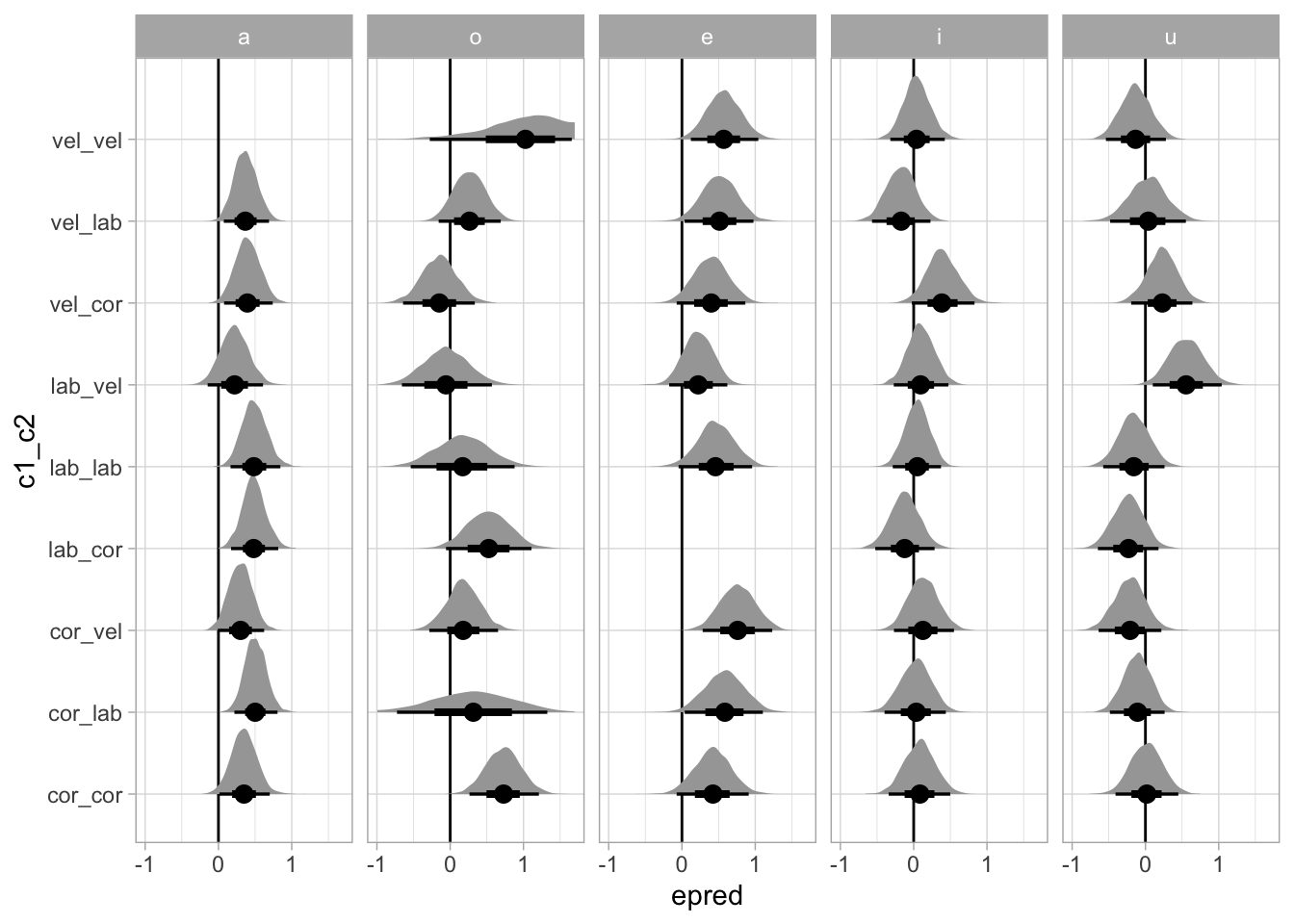

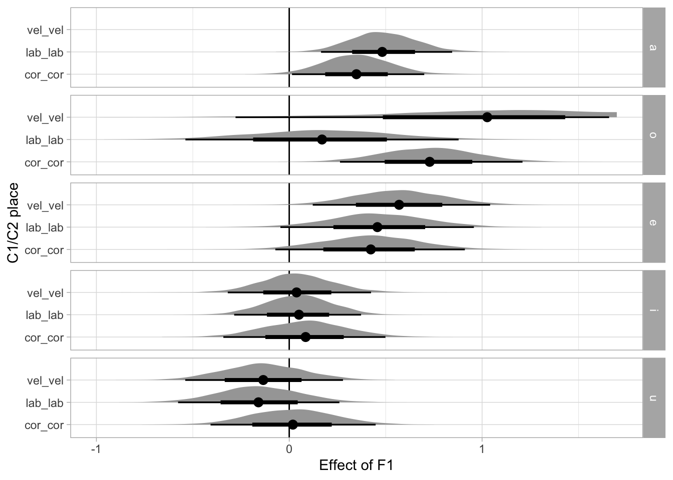
This is the same plot as above but including only homorganic place combinations.

bm_1_draws_long_avg_pl_vow |> 
  filter(coef == "b", !(c1_c2 == "lab_cor" & vowel == "e"), !(c1_c2 == "vel_vel" & vowel == "a"), c1_c2 %in% c("lab_lab", "cor_cor", "vel_vel")) |> 
  mutate(vowel = factor(vowel, levels = c("a", "o", "e", "i", "u"))) |> 
  ggplot(aes(epred, c1_c2)) +
  geom_vline(xintercept = 0) +
  stat_halfeye() +
  facet_grid(rows = vars(vowel)) +
  xlim(-1, 1.7) +
  labs(
    x = "Effect of F1", y = "C1/C2 place"
  )

ggsave("img/bm1-f1-place.png", width = 5, height = 5)

4.4 Coefficient tables

The following table shows 95, 90, 80 and 60% CrI for the a coefficient by vowel (the intercept by vowel).

bm_1_coef_table_a <- bm_1_draws_long_avg |>
  filter(coef == "a") |> 
  group_by(vowel) |> 
  reframe(
    q95 = round(quantile2(epred, probs = c(0.025, 0.975)), 2),
    q90 = round(quantile2(epred, probs = c(0.05, 0.95)), 2),
    q80 = round(quantile2(epred, probs = c(0.1, 0.9)), 2),
    q60 = round(quantile2(epred, probs = c(0.2, 0.8)), 2)
  ) |> 
  mutate(limit = rep(c("lo", "hi"), length.out = n())) |> 
  pivot_wider(names_from = limit, values_from = q95:q60) |> 
  unite("q95", q95_lo, q95_hi, sep = ", ") |> 
  unite("q90", q90_lo, q90_hi, sep = ", ") |> 
  unite("q80", q80_lo, q80_hi, sep = ", ") |> 
  unite("q60", q60_lo, q60_hi, sep = ", ")
bm_1_coef_table_a

# A tibble: 5 × 5
  vowel q95          q90          q80          q60         
  <chr> <chr>        <chr>        <chr>        <chr>       
1 a     -0.19, 0.41  -0.14, 0.36  -0.09, 0.31  -0.02, 0.24 
2 e     -0.06, 0.41  -0.02, 0.37  0.03, 0.33   0.08, 0.28  
3 i     -0.77, -0.54 -0.74, -0.55 -0.72, -0.58 -0.7, -0.6  
4 o     0.15, 0.42   0.17, 0.4    0.2, 0.37    0.23, 0.34  
5 u     -0.46, -0.16 -0.44, -0.19 -0.41, -0.21 -0.37, -0.25

# bm_1_coef_table_a |> knitr::kable(format = "latex") |> cat(sep = "\n")

The following table shows 95, 90, 80 and 60% CrI for the b coefficient by vowel and C1/C2 place (the effect of F1).

bm_1_coef_table_b_2 <- bm_1_draws_long_avg_pl_vow |>
  filter(coef == "b") |> 
  group_by(vowel, c1_c2) |> 
  reframe(
    q95 = round(quantile2(epred, probs = c(0.025, 0.975)), 2),
    q90 = round(quantile2(epred, probs = c(0.05, 0.95)), 2),
    q80 = round(quantile2(epred, probs = c(0.1, 0.9)), 2),
    q60 = round(quantile2(epred, probs = c(0.2, 0.8)), 2)
  ) |> 
  mutate(limit = rep(c("lo", "hi"), length.out = n())) |> 
  pivot_wider(names_from = limit, values_from = q95:q60) |> 
  unite("q95", q95_lo, q95_hi, sep = ", ") |> 
  unite("q90", q90_lo, q90_hi, sep = ", ") |> 
  unite("q80", q80_lo, q80_hi, sep = ", ") |> 
  unite("q60", q60_lo, q60_hi, sep = ", ")
bm_1_coef_table_b_2

# A tibble: 45 × 6
   vowel c1_c2   q95         q90         q80         q60        
   <chr> <chr>   <chr>       <chr>       <chr>       <chr>      
 1 a     cor_cor 0.01, 0.7   0.07, 0.63  0.13, 0.57  0.2, 0.49  
 2 a     cor_lab 0.22, 0.81  0.27, 0.75  0.32, 0.69  0.38, 0.63 
 3 a     cor_vel -0.01, 0.62 0.04, 0.57  0.09, 0.51  0.16, 0.44 
 4 a     lab_cor 0.17, 0.82  0.22, 0.76  0.28, 0.7   0.35, 0.61 
 5 a     lab_lab 0.17, 0.84  0.22, 0.77  0.27, 0.71  0.34, 0.63 
 6 a     lab_vel -0.15, 0.61 -0.09, 0.55 -0.03, 0.47 0.06, 0.38 
 7 a     vel_cor 0.08, 0.74  0.12, 0.68  0.18, 0.62  0.25, 0.54 
 8 a     vel_lab 0.07, 0.69  0.11, 0.64  0.17, 0.58  0.24, 0.5  
 9 a     vel_vel -1.97, 1.94 -1.66, 1.65 -1.27, 1.29 -0.84, 0.83
10 e     cor_cor -0.07, 0.91 0.01, 0.83  0.1, 0.74   0.21, 0.63 
# ℹ 35 more rows

# bm_1_coef_table_b_2 |> knitr::kable(format = "latex") |> cat(sep = "\n")

4.5 Posterior predictive check and sensitivity analysis

Posterior predictive checks are good.

pp_check(bm_1, ndraws = 50)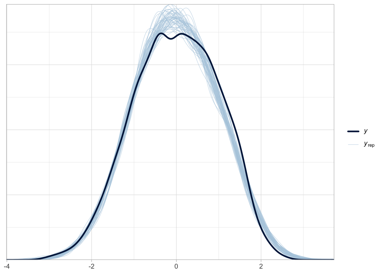

bm_1_fix <- fixef(bm_1) |> as_tibble(rownames = "term") |> 
  mutate(
    theta = rep(0, 91),
    sigma_prior = c(rep(1, 90), 0.1),
    z = abs((Estimate - theta) / Est.Error),
    s = 1 - (Est.Error^2 / sigma_prior^2),
    term = str_remove(term, "vowel") |> str_remove_all("(c1|c2)_place")
  )

labels <- tibble(
  s = c(0.25, 0.25, 0.75, 0.75),
  z = c(1.25, 3.75, 1.25, 3.75),
  term = c("Poorly identified", "Prior/Posterior\nconflict", "Ideal", "Overfit")
)

bm_1_fix |> 
  ggplot(aes(s, z, label = term)) +
  annotate("rect", xmin = 0, ymin = 0, xmax = 0.5, ymax = 2.5, alpha = 0.5, fill = "#e66101") +
  annotate("rect", xmin = 0, ymin = 2.5, xmax = 0.5, ymax = Inf, alpha = 0.5, fill = "#fdb863") +
  annotate("rect", xmin = 0.5, ymin = 0, xmax = 1, ymax = 2.5, alpha = 0.5, fill = "#b2abd2") +
  annotate("rect", xmin = 0.5, ymin = 2.5, xmax = 1, ymax = Inf, alpha = 0.5, fill = "#5e3c99") +
  geom_text(size = 3, alpha = 0.5) +
  # geom_point(alpha = 0.5) +
  geom_label(data = labels, colour = "white", fill = "black") +
  xlim(0, 1)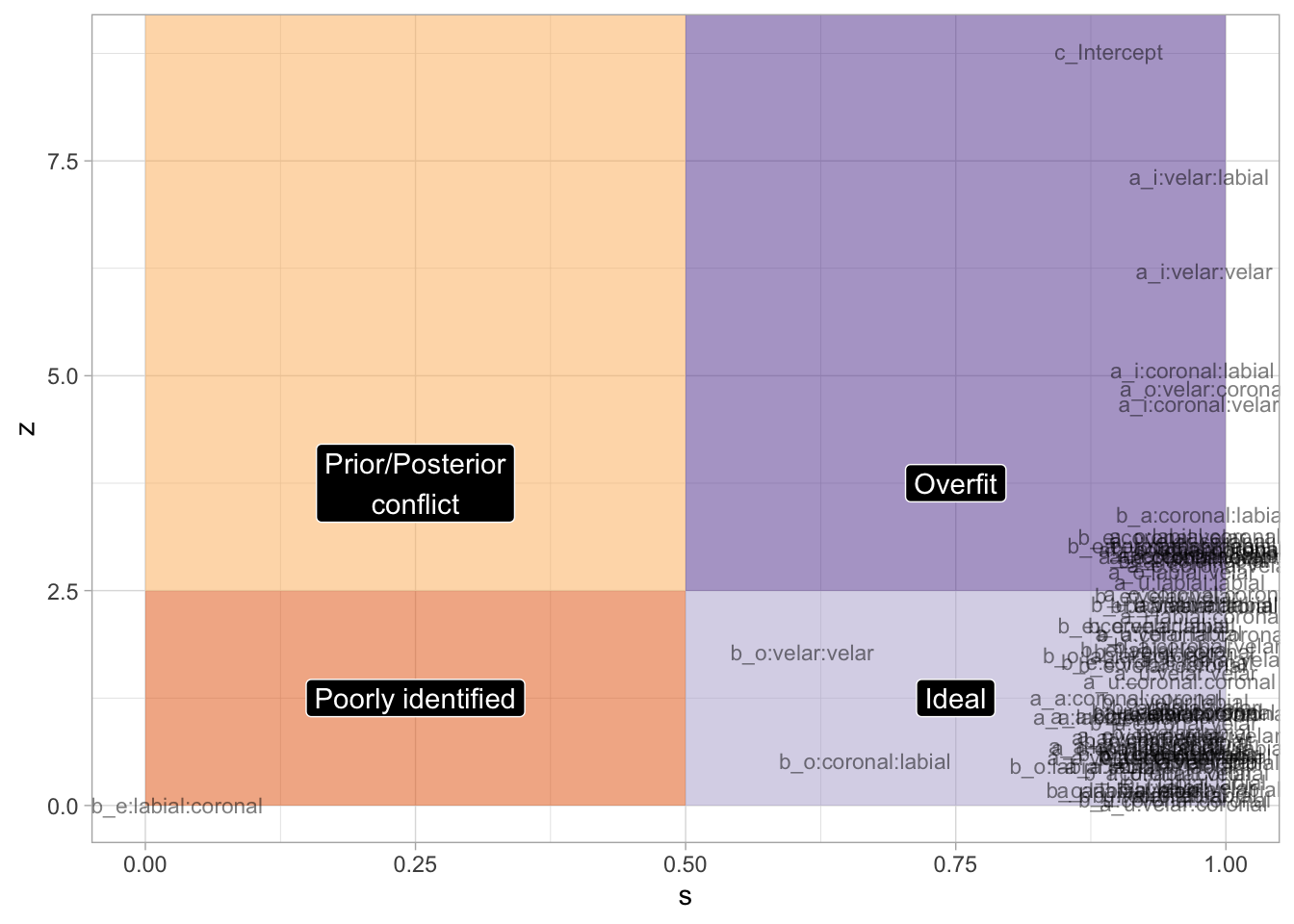

4.6 Model plotting

We need to get the predicted draws to convert duration and F1 back to ms and hz. Note that duration was logged then scaled.

seq_minmax <- function(x, by = 1) {
  seq(min(x), max(x), by = by)
}

bm_1_preds <- bm_1_draws_long |> 
  group_by(coef, vowel, .draw) |> 
  summarise(
    value = mean(value),
    .groups = "drop"
  ) |> 
  pivot_wider(names_from = coef, values_from = value) |> 
  mutate(
    f13_z = list(seq_minmax(ita_egg$f13_z, 0.5))
  ) |> 
  unnest_longer(f13_z) |> 
  mutate(
    epred = a + b * f13_z,
    duration_log = epred * sd(ita_egg$duration_log) + mean(ita_egg$duration_log),
    duration = exp(duration_log),
    f13 = f13_z * sd(ita_egg$f13) + mean(ita_egg$f13),
    vowel = str_remove(vowel, "vowel")
  )

Let’s also calculate the mean F1 values for each vowel, to be added in the plot below.

vmean_f13 <- ita_egg |>
  group_by(vowel) |>
  summarise(f13_mean = mean(f13))
vmean_f13z <- ita_egg |>
  group_by(vowel) |>
  summarise(f13z_mean = mean(f13_z))

We can now plot the model predictions in the original scale.

bm_1_preds |>
  group_by(vowel, f13) |>
  summarise(
    duration_ms = median(duration),
    # Get the 90% CrI
    q0.05 = quantile(duration, probs = 0.05),
    q0.90 = quantile(duration, probs = 0.95),
    .groups = "drop"
  ) |>
  ggplot(aes(f13, duration_ms)) +
  geom_ribbon(aes(ymin = q0.05, ymax = q0.90, fill = vowel), alpha = 0.25) +
  geom_line(aes(colour = vowel), linewidth = 1) +
  facet_wrap(~vowel) +
  scale_colour_viridis_d() +
  scale_fill_viridis_d()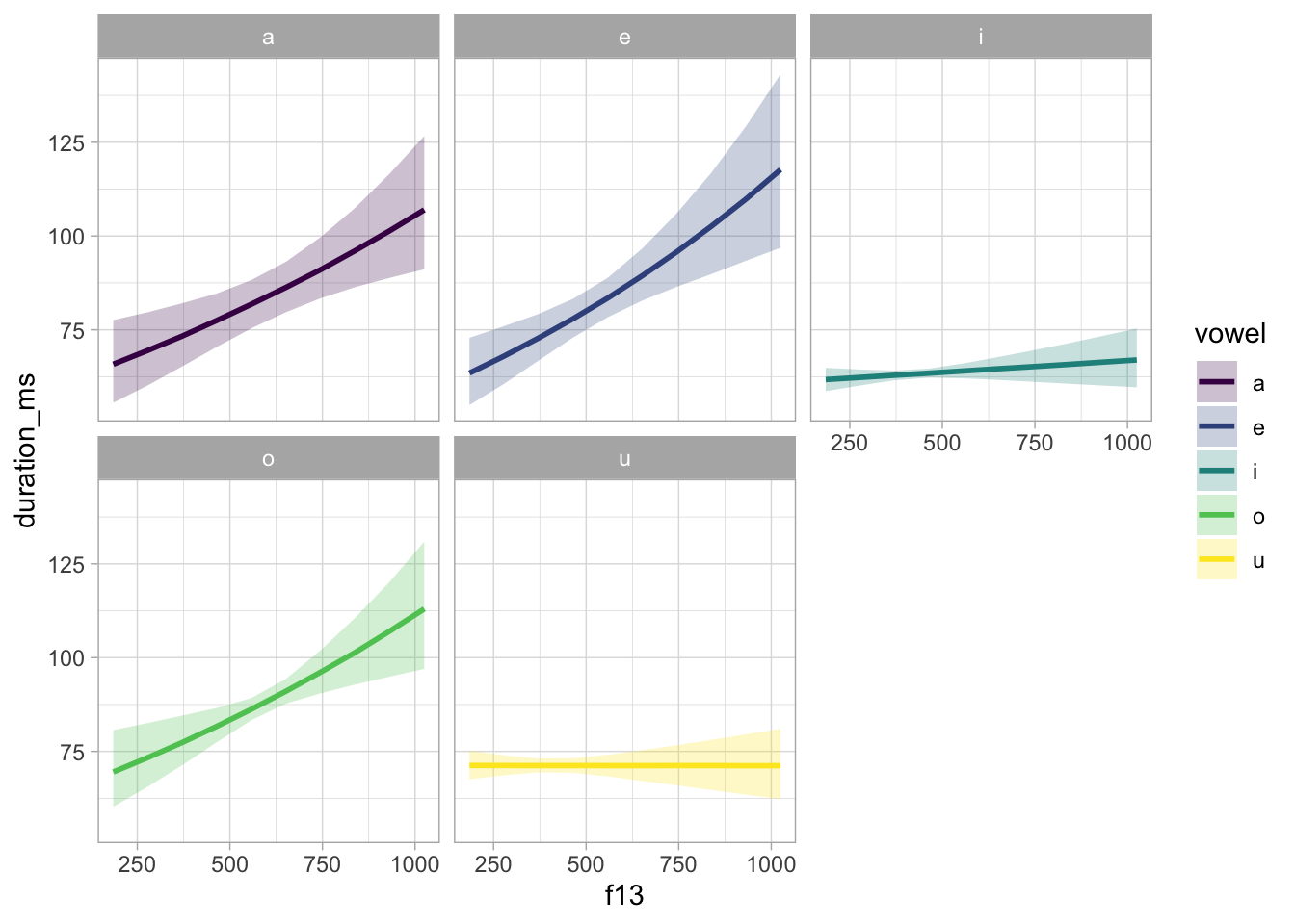

bm_1_preds |>
  group_by(vowel, f13) |>
  ggplot(aes(f13, duration)) +
  stat_lineribbon() +
  facet_wrap(~vowel) +
  scale_fill_brewer()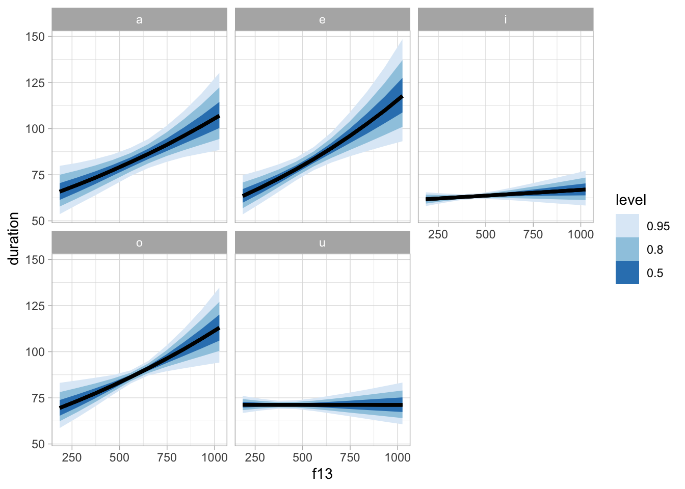

bm_1_preds |>
  mutate(
    vowel = str_replace(vowel, "o", "ɔ"),
    vowel = factor(vowel, levels = c("i", "u", "e", "ɔ", "a"))
  ) |> 
  group_by(vowel, f13) |>
  ggplot(aes(f13, duration, fill = vowel)) +
  stat_ribbon(.width = 0.98, alpha = 0.2) +
  stat_ribbon(.width = 0.9, alpha = 0.4) +
  stat_lineribbon(.width = 0.6, alpha = 0.8) +
  geom_vline(data = vmean_f13 |>   mutate(
    vowel = str_replace(vowel, "o", "ɔ"),
    vowel = factor(vowel, levels = c("i", "u", "e", "ɔ", "a"))
  ), aes(xintercept = f13_mean, colour = vowel), linetype = "dashed") +
  geom_rug(data = ita_egg |>   mutate(
    vowel = str_replace(vowel, "o", "ɔ"),
    vowel = factor(vowel, levels = c("i", "u", "e", "ɔ", "a"))
  ), alpha = 0.1, length = unit(0.015, "npc"), aes(colour = vowel)) +
  facet_wrap(~vowel) +
  labs(
    x = "F1 (Hz)", y = "Duration (ms)"
  ) +
  scale_fill_manual(values = cols) +
  scale_color_manual(values = cols) +
  theme(legend.position = "none")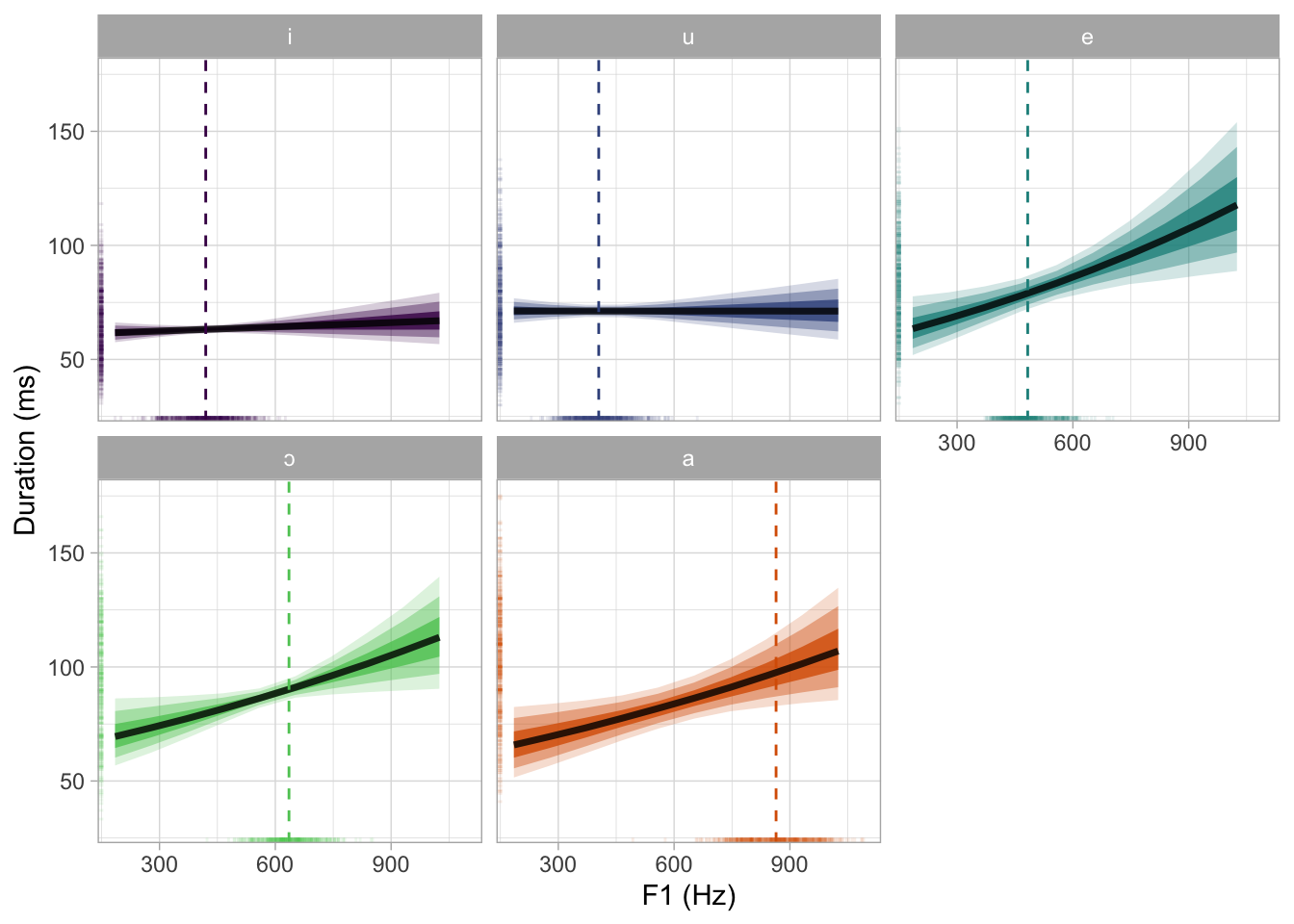

ggsave("img/bm1-pred-plot-ms-hz.png", width = 7, height = 5)

But let’s also plot this in the standardised logged duration scale.

bm_1_preds |>
  group_by(vowel, f13) |>
  ggplot(aes(f13_z, epred, fill = vowel)) +
  stat_ribbon(.width = 0.98, alpha = 0.2) +
  stat_ribbon(.width = 0.9, alpha = 0.4) +
  stat_lineribbon(.width = 0.6, alpha = 0.8) +
  geom_vline(data = vmean_f13z, aes(xintercept = f13z_mean, colour = vowel)) +
  facet_wrap(~vowel) +
  scale_fill_viridis_d()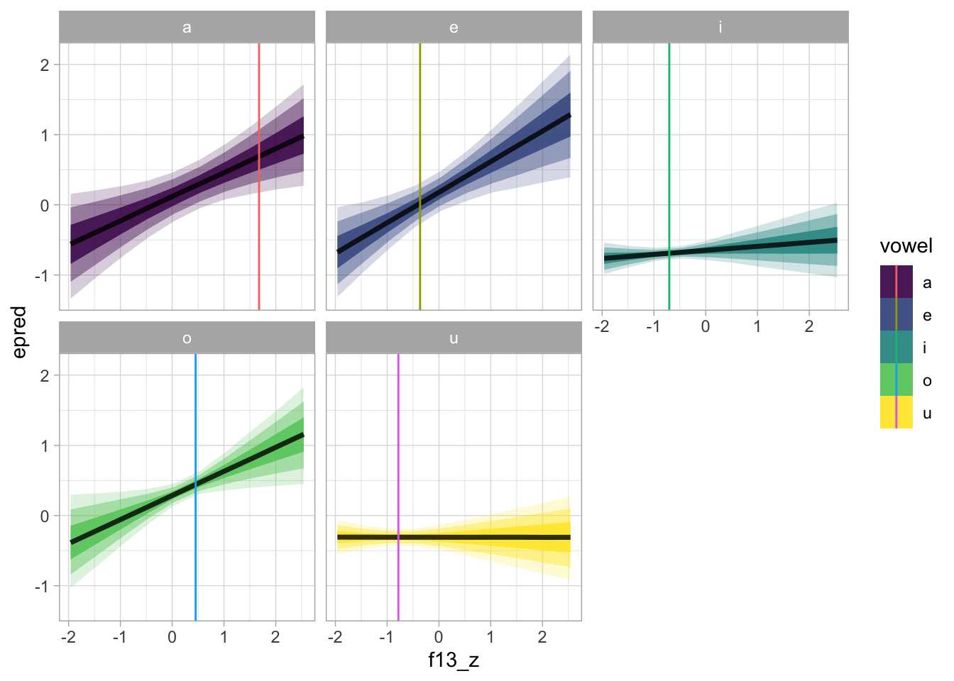

4.7 Group-level effects

bm_1_ranef <- bm_1 |>
  gather_draws(r_speaker__c[subject,var])

bm_1_ranef |>
  ggplot(aes(y = reorder(subject, .value, median), x = .value)) +
  geom_vline(xintercept = 0) +
  stat_halfeye()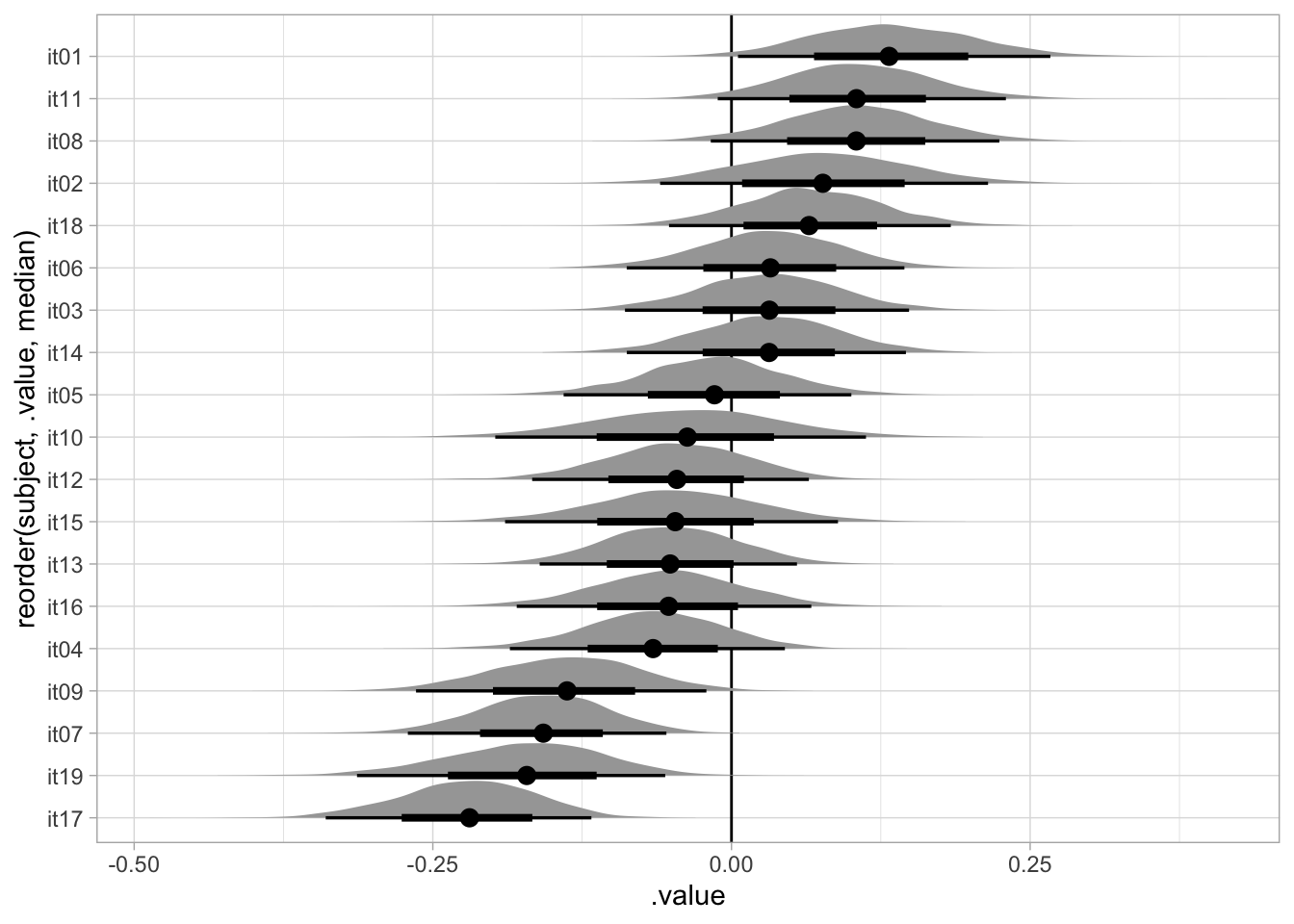

5 Non-linear modelling: GAM

A GAM model with the mgcv package is run to get an estimate number of k since brms does not optimise k and fits the model just with the default k which can slow down the MCMC sampling with large values of k.

gam_1 <- bam(
  duration_logz ~
    vowel +
    s(f13_z) +
    s(f13_z, speaker, by = vowel, bs = "fs", m = 1) +
    s(speech_rate_logz) +
    s(speech_rate_logz, speaker, bs = "fs", m = 1),
  data = ita_egg
)

Warning in gam.side(sm, X, tol = .Machine$double.eps^0.5): model has repeated
1-d smooths of same variable.

summary(gam_1)

Family: gaussian 
Link function: identity 

Formula:
duration_logz ~ vowel + s(f13_z) + s(f13_z, speaker, by = vowel, 
    bs = "fs", m = 1) + s(speech_rate_logz) + s(speech_rate_logz, 
    speaker, bs = "fs", m = 1)

Parametric coefficients:
            Estimate Std. Error t value Pr(>|t|)    
(Intercept)  0.10762    0.14848   0.725   0.4686    
vowele       0.05915    0.14477   0.409   0.6829    
voweli      -0.59166    0.15070  -3.926 8.83e-05 ***
vowelo       0.28281    0.12060   2.345   0.0191 *  
vowelu      -0.22071    0.16073  -1.373   0.1698    
---
Signif. codes:  0 '***' 0.001 '**' 0.01 '*' 0.05 '.' 0.1 ' ' 1

Approximate significance of smooth terms:
                               edf  Ref.df      F  p-value    
s(f13_z)                     3.484   4.235 12.819  < 2e-16 ***
s(f13_z,speaker):vowela     16.684 144.000  0.346  < 2e-16 ***
s(f13_z,speaker):vowele     17.048 137.000  0.247 1.19e-06 ***
s(f13_z,speaker):voweli     11.431 148.000  0.121 3.31e-05 ***
s(f13_z,speaker):vowelo     18.291 147.000  0.315  < 2e-16 ***
s(f13_z,speaker):vowelu     24.993 151.000  0.606  < 2e-16 ***
s(speech_rate_logz)          4.183   4.948 20.333  < 2e-16 ***
s(speech_rate_logz,speaker) 52.949 170.000  2.523  < 2e-16 ***
---
Signif. codes:  0 '***' 0.001 '**' 0.01 '*' 0.05 '.' 0.1 ' ' 1

R-sq.(adj) =  0.742   Deviance explained = 75.5%
fREML = 2415.4  Scale est. = 0.2583    n = 3019

vmean <- aggregate(ita_egg$f13_z, list(ita_egg$vowel), mean)
# fs_terms <- c("s(f13_z,speaker)")
fs_terms <- c("s(f13_z,speaker):vowela", "s(f13_z,speaker):vowele", "s(f13_z,speaker):voweli", "s(f13_z,speaker):vowelo", "s(f13_z,speaker):vowelu", "s(speech_rate_logz,speaker)")

predict_gam(gam_1, exclude_terms = fs_terms, length_out = 100, values = list(speech_rate_logz = 0)) |>
  plot(series = "f13_z", comparison = "vowel") +
  geom_vline(data = vmean, aes(xintercept = x, colour = Group.1)) +
  geom_hline(yintercept = 0, linetype = "dashed") +
  facet_wrap(~vowel)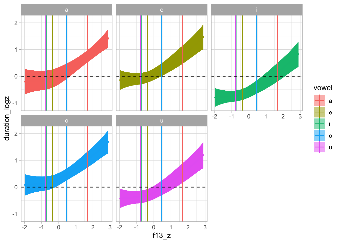

6 Non-linear modelling: BRM

6.1 Prior predictive checks

priors_s <- c(
  prior(normal(0, 1), class = b),
  prior(cauchy(0, 0.01), class = sigma),
  prior(cauchy(0, 1), class = sds)
)

bms_1_f <- bf(
  duration_logz ~
    0 + vowel +
    s(f13_z, k = 5) +
    s(f13_z, speaker, by = vowel, bs = "fs", m = 1) +
    s(speech_rate_logz, k = 5) +
    s(speech_rate_logz, speaker, bs = "fs", m = 1)
)

bms_1_priors <- brm(
  bms_1_f,
  family = gaussian,
  data = ita_egg,
  prior = priors_s,
  sample_prior = "only",
  cores = 4,
  threads = threading(2),
  backend = "cmdstanr",
  file = "data/cache/bms_1_priors",
  seed = my_seed
)

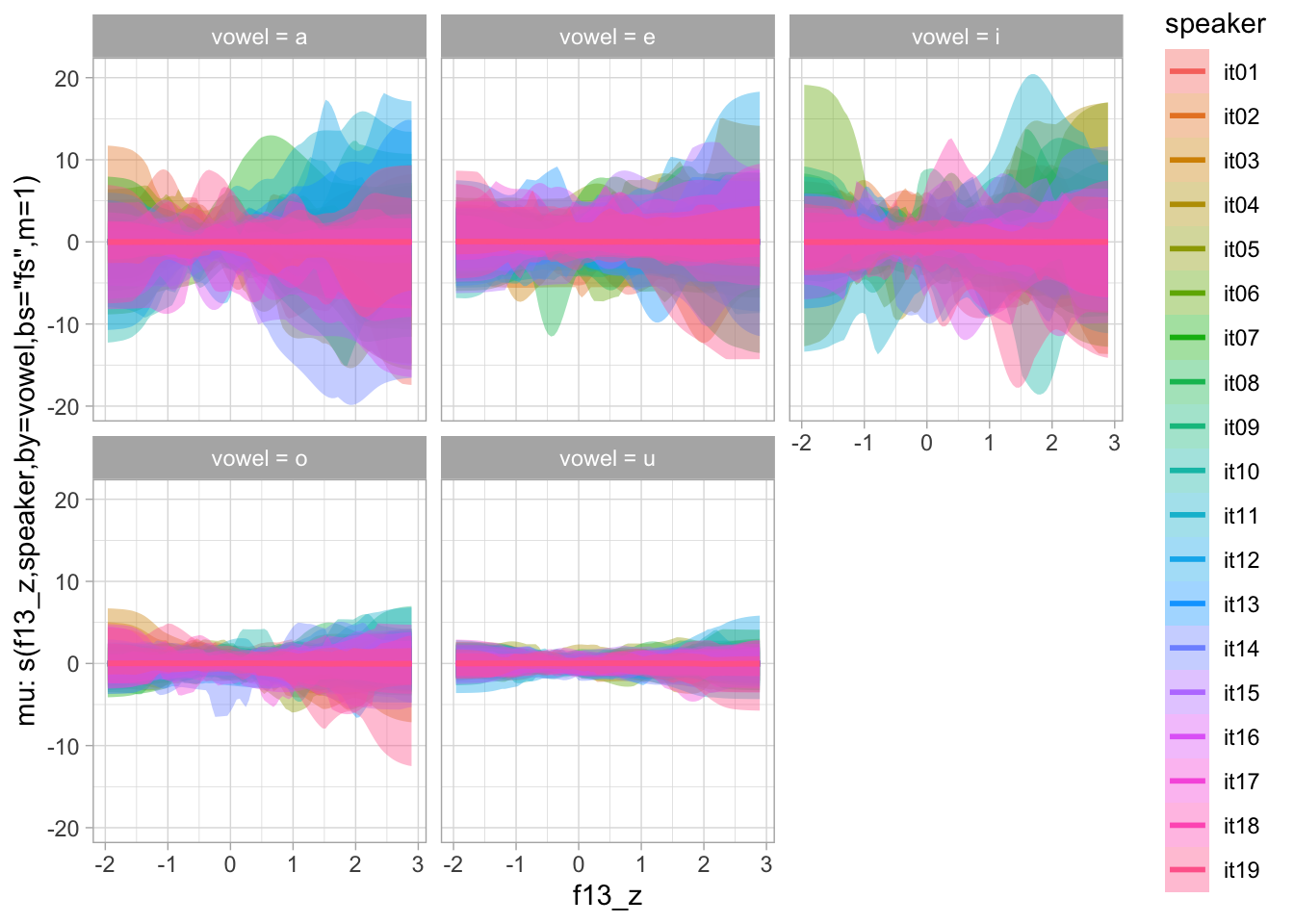
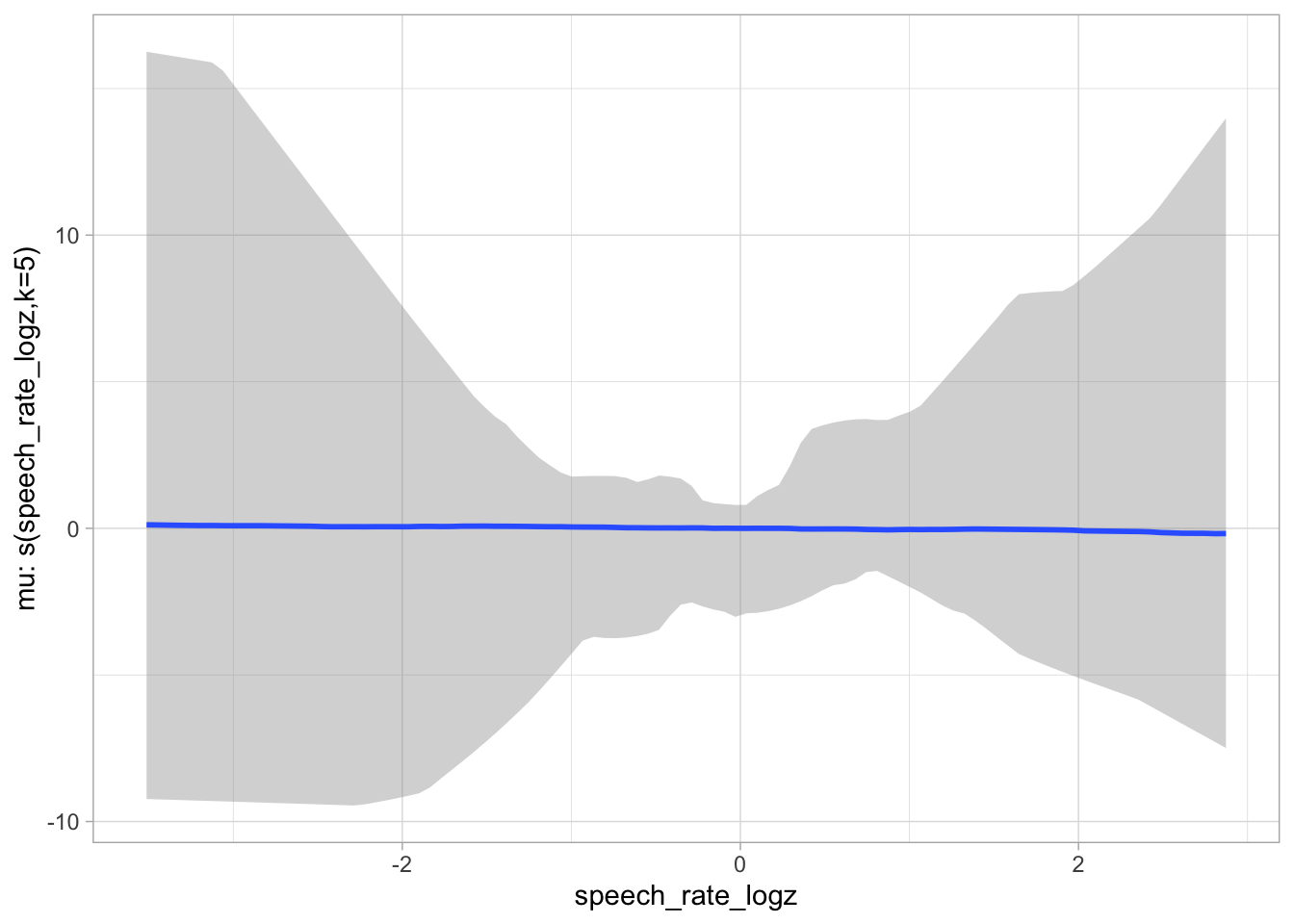
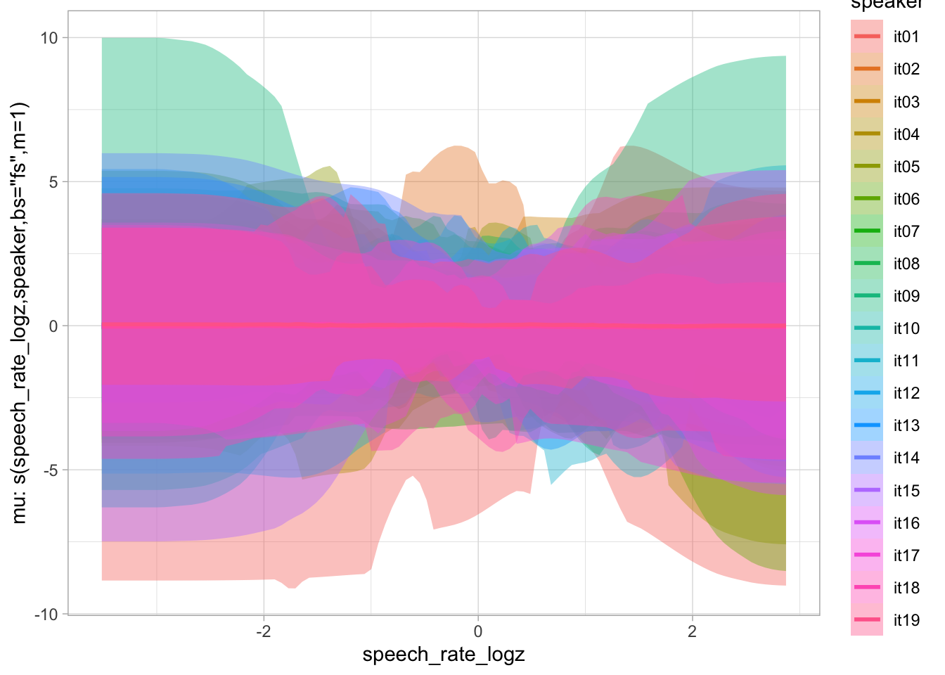
plot(conditional_smooths(bms_1_priors, ndraws = 100), ask = FALSE)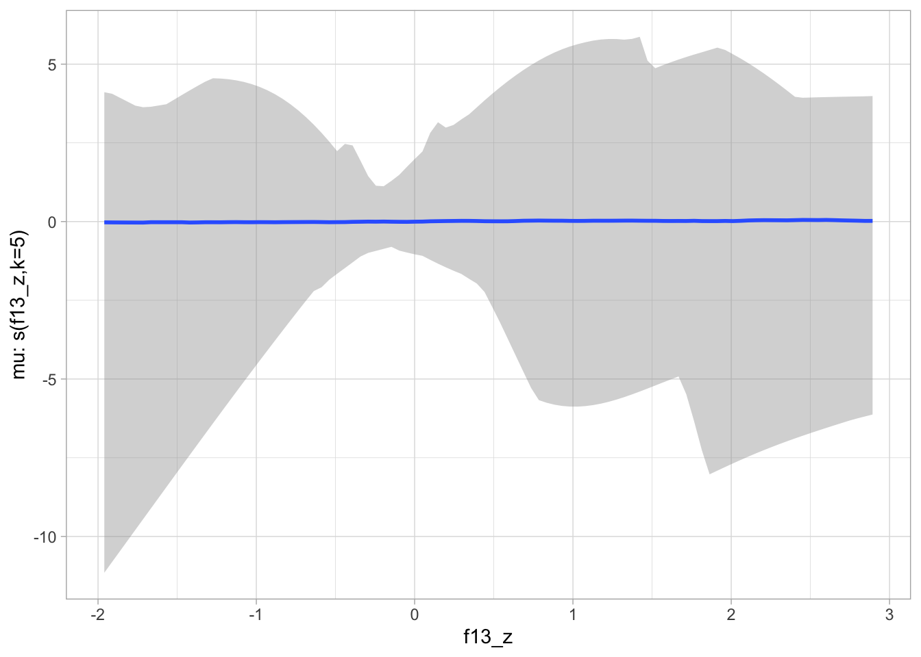

6.2 Model fit

We specify k = 5 based on the mgcv modelling above. Reducing k speeds up estimation (because there are less basis functions, hence less parameters to estimate).

The model takes about 4-5 hours to run on 8 cores.

bms_1 <- brm(
  bms_1_f,
  family = gaussian,
  data = ita_egg,
  prior = priors_s,
  cores = 4,
  threads = threading(2),
  backend = "cmdstanr",
  file = "data/cache/bms_1",
  seed = my_seed
)

summary(bms_1, prob = 0.9)

 Family: gaussian 
  Links: mu = identity; sigma = identity 
Formula: duration_logz ~ 0 + vowel + s(f13_z, k = 5) + s(f13_z, speaker, by = vowel, bs = "fs", m = 1) + s(speech_rate_logz, k = 5) + s(speech_rate_logz, speaker, bs = "fs", m = 1) 
   Data: ita_egg (Number of observations: 3019) 
  Draws: 4 chains, each with iter = 2000; warmup = 1000; thin = 1;
         total post-warmup draws = 4000

Smoothing Spline Hyperparameters:
                                Estimate Est.Error l-90% CI u-90% CI Rhat
sds(sf13_z_1)                       1.57      0.87     0.69     3.22 1.00
sds(sf13_zspeakervowela_1)          0.34      0.23     0.03     0.76 1.00
sds(sf13_zspeakervowela_2)          1.90      1.96     0.08     6.11 1.01
sds(sf13_zspeakervowele_1)          0.33      0.22     0.03     0.74 1.00
sds(sf13_zspeakervowele_2)          1.93      1.96     0.09     6.17 1.00
sds(sf13_zspeakervoweli_1)          0.33      0.22     0.02     0.74 1.01
sds(sf13_zspeakervoweli_2)          1.99      2.03     0.09     6.40 1.00
sds(sf13_zspeakervowelo_1)          0.34      0.23     0.03     0.75 1.01
sds(sf13_zspeakervowelo_2)          1.82      1.90     0.09     5.93 1.00
sds(sf13_zspeakervowelu_1)          0.32      0.23     0.03     0.74 1.01
sds(sf13_zspeakervowelu_2)          2.04      2.03     0.08     6.17 1.01
sds(sspeech_rate_logz_1)            0.45      0.44     0.03     1.23 1.00
sds(sspeech_rate_logzspeaker_1)     0.78      0.13     0.58     1.00 1.00
sds(sspeech_rate_logzspeaker_2)     1.86      1.93     0.08     5.95 1.01
                                Bulk_ESS Tail_ESS
sds(sf13_z_1)                       2051     2236
sds(sf13_zspeakervowela_1)           492     1166
sds(sf13_zspeakervowela_2)           721     1055
sds(sf13_zspeakervowele_1)           562      884
sds(sf13_zspeakervowele_2)           818     1027
sds(sf13_zspeakervoweli_1)           404     1003
sds(sf13_zspeakervoweli_2)           607      802
sds(sf13_zspeakervowelo_1)           336      990
sds(sf13_zspeakervowelo_2)           581      909
sds(sf13_zspeakervowelu_1)           509      890
sds(sf13_zspeakervowelu_2)           619     1091
sds(sspeech_rate_logz_1)            1715     2314
sds(sspeech_rate_logzspeaker_1)     1573     2465
sds(sspeech_rate_logzspeaker_2)      825     1429

Regression Coefficients:
                    Estimate Est.Error l-90% CI u-90% CI Rhat Bulk_ESS Tail_ESS
vowela                  0.08      0.15    -0.16     0.32 1.00     2140     2459
vowele                  0.23      0.11     0.05     0.42 1.00     1266     1664
voweli                 -0.46      0.11    -0.64    -0.28 1.00     1300     1635
vowelo                  0.39      0.11     0.20     0.57 1.00     1299     1750
vowelu                 -0.10      0.11    -0.28     0.08 1.00     1271     1729
sf13_z_1                0.97      0.62    -0.04     1.98 1.00     3746     3388
sspeech_rate_logz_1    -2.57      0.42    -3.25    -1.89 1.00     2522     2503

Further Distributional Parameters:
      Estimate Est.Error l-90% CI u-90% CI Rhat Bulk_ESS Tail_ESS
sigma     0.52      0.01     0.51     0.53 1.00     5481     2619

Draws were sampled using sample(hmc). For each parameter, Bulk_ESS
and Tail_ESS are effective sample size measures, and Rhat is the potential
scale reduction factor on split chains (at convergence, Rhat = 1).

bms_1_coef_table <- bms_1 |>
  as_draws_df() |>
  select(b_vowela:b_vowelu) |>
  pivot_longer(b_vowela:b_vowelu) |>
  group_by(name) |>
  median_hdi()

Warning: Dropping 'draws_df' class as required metadata was removed.

bms_1_coef_table

# A tibble: 5 × 7
  name       value  .lower .upper .width .point .interval
  <chr>      <dbl>   <dbl>  <dbl>  <dbl> <chr>  <chr>    
1 b_vowela  0.0797 -0.197   0.368   0.95 median hdi      
2 b_vowele  0.234   0.0219  0.457   0.95 median hdi      
3 b_voweli -0.459  -0.678  -0.241   0.95 median hdi      
4 b_vowelo  0.386   0.175   0.612   0.95 median hdi      
5 b_vowelu -0.100  -0.306   0.131   0.95 median hdi      

# bms_1_coef_table |> knitr::kable(format = "latex") |> cat(sep = "\n")

bms_1_coef_table_2 <- bms_1 |>
  as_draws_df() |>
  select(b_vowela:b_vowelu) |>
  pivot_longer(b_vowela:b_vowelu) |>
  group_by(name) |>
  reframe(
    q95 = round(quantile2(value, probs = c(0.025, 0.975)), 2),
    q90 = round(quantile2(value, probs = c(0.05, 0.95)), 2),
    q80 = round(quantile2(value, probs = c(0.1, 0.9)), 2),
    q60 = round(quantile2(value, probs = c(0.2, 0.8)), 2)
  ) |> 
  mutate(limit = rep(c("lo", "hi"), length.out = n())) |> 
  pivot_wider(names_from = limit, values_from = q95:q60) |> 
  unite("q95", q95_lo, q95_hi, sep = ", ") |> 
  unite("q90", q90_lo, q90_hi, sep = ", ") |> 
  unite("q80", q80_lo, q80_hi, sep = ", ") |> 
  unite("q60", q60_lo, q60_hi, sep = ", ")

Warning: Dropping 'draws_df' class as required metadata was removed.

bms_1_coef_table_2

# A tibble: 5 × 5
  name     q95          q90          q80         q60         
  <chr>    <chr>        <chr>        <chr>       <chr>       
1 b_vowela -0.22, 0.36  -0.16, 0.32  -0.11, 0.27 -0.04, 0.2  
2 b_vowele 0.02, 0.45   0.05, 0.42   0.09, 0.37  0.14, 0.32  
3 b_voweli -0.68, -0.24 -0.64, -0.28 -0.6, -0.32 -0.55, -0.37
4 b_vowelo 0.16, 0.61   0.2, 0.57    0.24, 0.53  0.3, 0.48   
5 b_vowelu -0.32, 0.12  -0.28, 0.08  -0.24, 0.04 -0.19, -0.01

# bms_1_coef_table_2 |> knitr::kable(format = "latex") |> cat(sep = "\n")

6.3 Posterior predictive check and sensitivity analysis

pp_check(bms_1, ndraws = 50)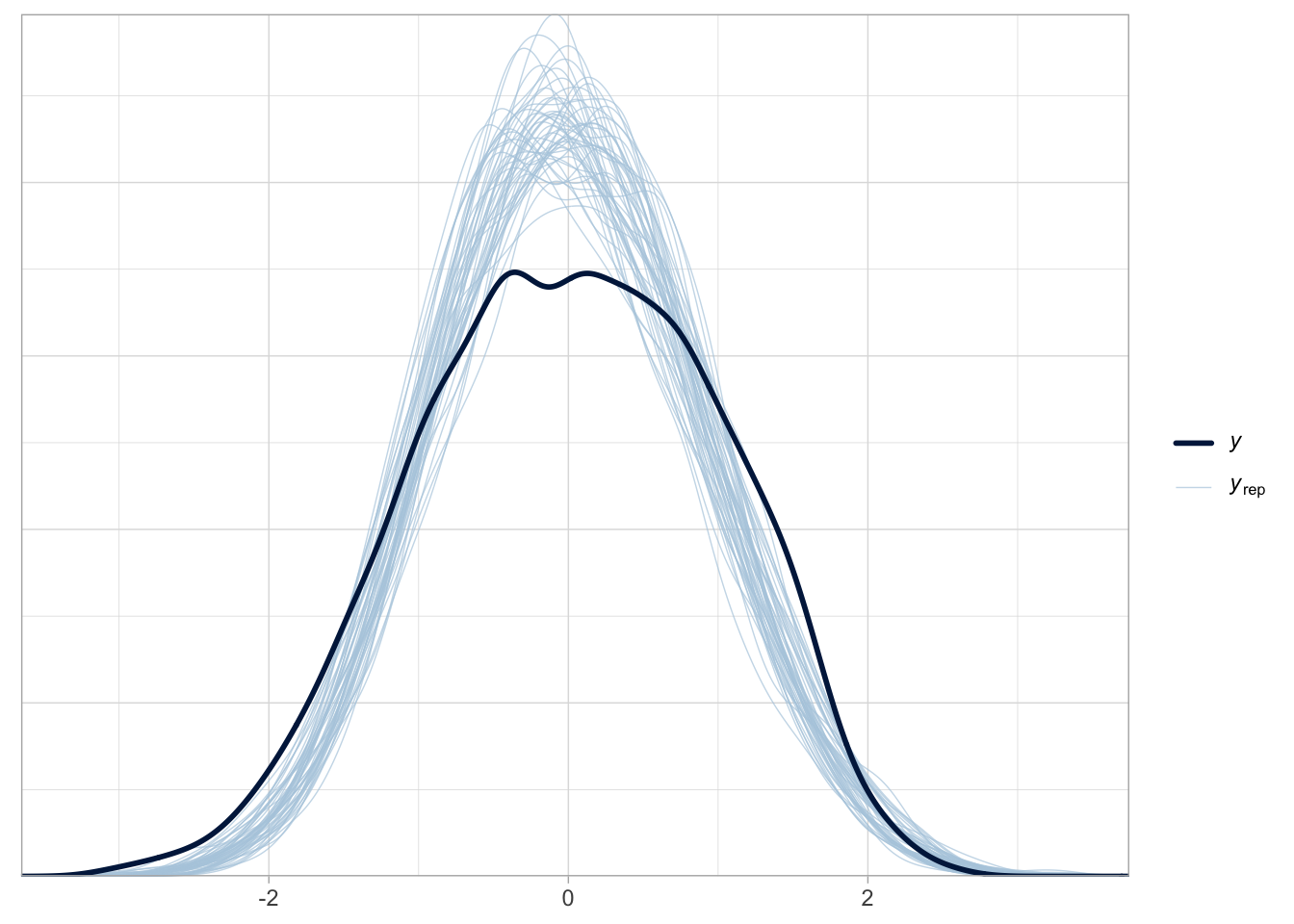

bms_1_fix <- fixef(bms_1) |> as_tibble(rownames = "term") |> 
  mutate(
    theta = rep(0, 7),
    sigma_prior = rep(1, 7),
    z = abs((Estimate - theta) / Est.Error),
    s = 1 - (Est.Error^2 / sigma_prior^2)
  )
bms_1_fix

# A tibble: 7 × 9
  term           Estimate Est.Error    Q2.5  Q97.5 theta sigma_prior     z     s
  <chr>             <dbl>     <dbl>   <dbl>  <dbl> <dbl>       <dbl> <dbl> <dbl>
1 vowela           0.0797     0.146 -0.215   0.358     0           1 0.547 0.979
2 vowele           0.235      0.110  0.0170  0.454     0           1 2.12  0.988
3 voweli          -0.460      0.111 -0.677  -0.240     0           1 4.16  0.988
4 vowelo           0.387      0.111  0.165   0.608     0           1 3.48  0.988
5 vowelu          -0.100      0.111 -0.320   0.123     0           1 0.901 0.988
6 sf13_z_1         0.971      0.621 -0.226   2.18      0           1 1.56  0.614
7 sspeech_rate_…  -2.57       0.420 -3.41   -1.74      0           1 6.11  0.823

labels <- tibble(
  s = c(0.25, 0.25, 0.75, 0.75),
  z = c(1.25, 3.75, 1.25, 3.75),
  term = c("Poorly identified", "Prior/Posterior\nconflict", "Ideal", "Overfit")
)

bms_1_fix |> 
  ggplot(aes(s, z, label = term)) +
  annotate("rect", xmin = 0, ymin = 0, xmax = 0.5, ymax = 2.5, alpha = 0.5, fill = "#e66101") +
  annotate("rect", xmin = 0, ymin = 2.5, xmax = 0.5, ymax = Inf, alpha = 0.5, fill = "#fdb863") +
  annotate("rect", xmin = 0.5, ymin = 0, xmax = 1, ymax = 2.5, alpha = 0.5, fill = "#b2abd2") +
  annotate("rect", xmin = 0.5, ymin = 2.5, xmax = 1, ymax = Inf, alpha = 0.5, fill = "#5e3c99") +
  geom_text() +
  geom_point() +
  geom_label(data = labels, colour = "white", fill = "black") +
  xlim(0, 1)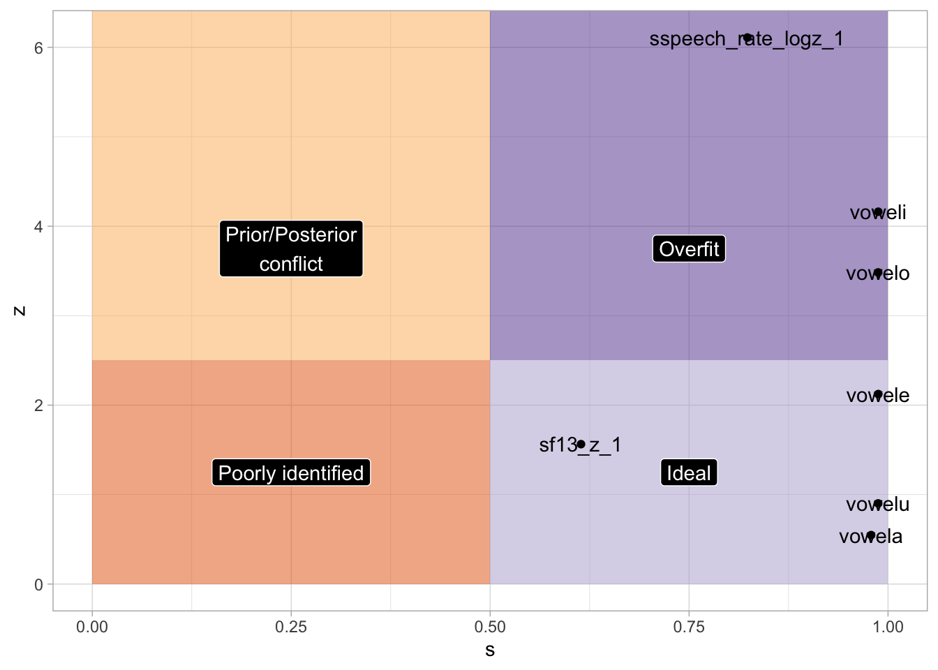

6.4 Model plotting

plot(conditional_effects(bms_1, "f13_z:vowel"), plot = FALSE)[[1]] + facet_wrap(~vowel)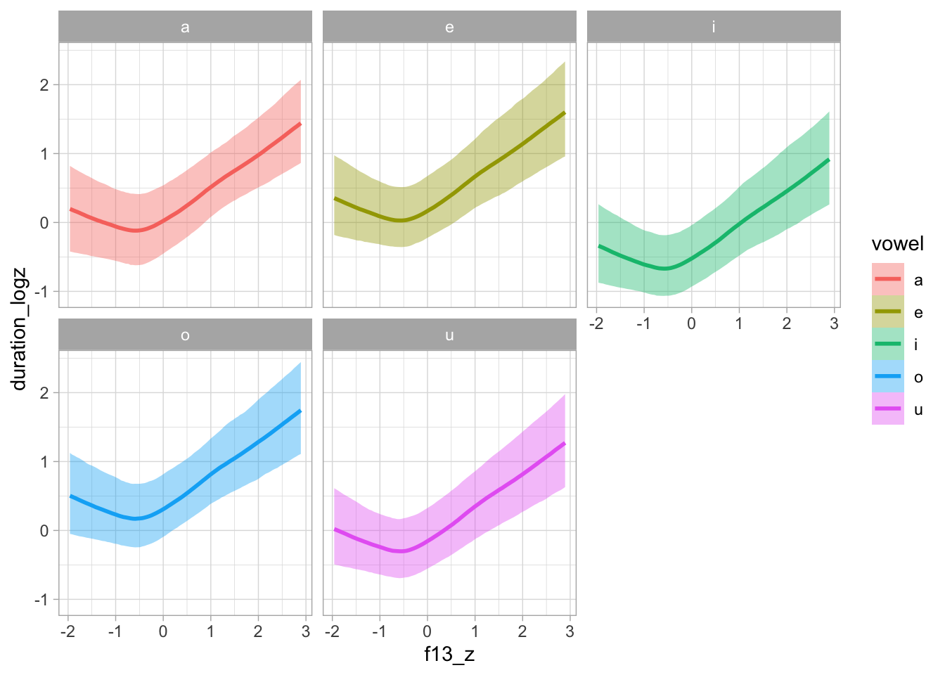

plot(conditional_effects(bms_1, "f13_z:vowel", spaghetti = TRUE, ndraws = 100), plot = FALSE)[[1]] + facet_wrap(~vowel)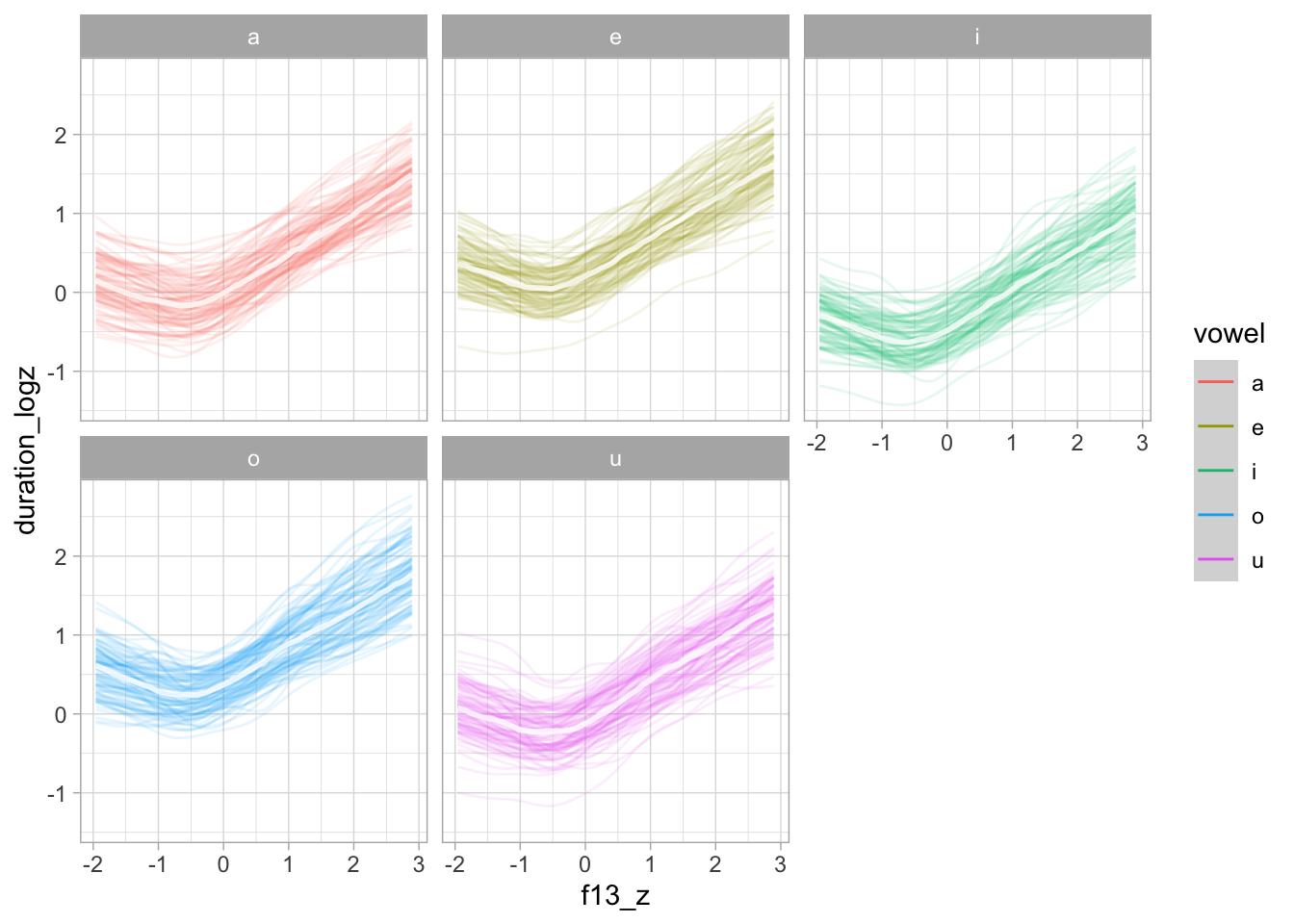

Let’s plot on the original scale.

seq_minmax <- function(x, by = 1) {
  seq(min(x), max(x), by = by)
}

bms_1_grid <- expand_grid(
  vowel = levels(ita_egg$vowel),
  f13_z = seq_minmax(ita_egg$f13_z, 0.25),
  speech_rate_logz = 0,
  speaker = NA
)

bms_1_preds <- epred_draws(bms_1, newdata = bms_1_grid, re_formula = NA) |>
  mutate(
    duration_log = .epred * sd(ita_egg$duration_log) + mean(ita_egg$duration_log),
    duration = exp(duration_log),
    f13 = f13_z * sd(ita_egg$f13) + mean(ita_egg$f13)
  )

bms_1_grid_m <- expand_grid(
  vowel = levels(ita_egg$vowel),
  f13_z = 0,
  speech_rate_logz = 0, 
  speaker = NA
)

bms_1_preds_m <- epred_draws(bms_1, newdata = bms_1_grid_m, re_formula = NA) |>
  mutate(
    duration_log = .epred * sd(ita_egg$duration_log) + mean(ita_egg$duration_log),
    duration = exp(duration_log),
    f13 = f13_z * sd(ita_egg$f13) + mean(ita_egg$f13)
  )

mean_pred_vdur <- round(mean(bms_1_preds_m$duration))

bms_1_preds |>
  mutate(
    vowel = str_replace(vowel, "o", "ɔ"),
    vowel = factor(vowel, levels = c("i", "u", "e", "ɔ", "a"))
  ) |> 
  group_by(vowel, f13) |>
  ggplot(aes(f13, duration, fill = vowel)) +
  geom_hline(yintercept = mean_pred_vdur, linetype = "dashed", colour = "red") +
  stat_ribbon(.width = 0.98, alpha = 0.2) +
  stat_ribbon(.width = 0.9, alpha = 0.4) +
  stat_lineribbon(.width = 0.6, alpha = 0.8) +
  geom_vline(data = vmean_f13 |>  mutate(
    vowel = str_replace(vowel, "o", "ɔ"),
    vowel = factor(vowel, levels = c("i", "u", "e", "ɔ", "a"))
  ), aes(xintercept = f13_mean, colour = vowel), linetype = "dashed") +
  geom_rug(data = ita_egg |> mutate(
    vowel = str_replace(vowel, "o", "ɔ"),
    vowel = factor(vowel, levels = c("i", "u", "e", "ɔ", "a"))
  ), alpha = 0.1, length = unit(0.015, "npc"), aes(colour = vowel)) +
  facet_wrap(~vowel) +
  labs(
    x = "F1 (Hz)", y = "Duration (ms)"
  ) +
  scale_fill_manual(values = cols) +
  scale_colour_manual(values = cols) +
  theme(legend.position = "none")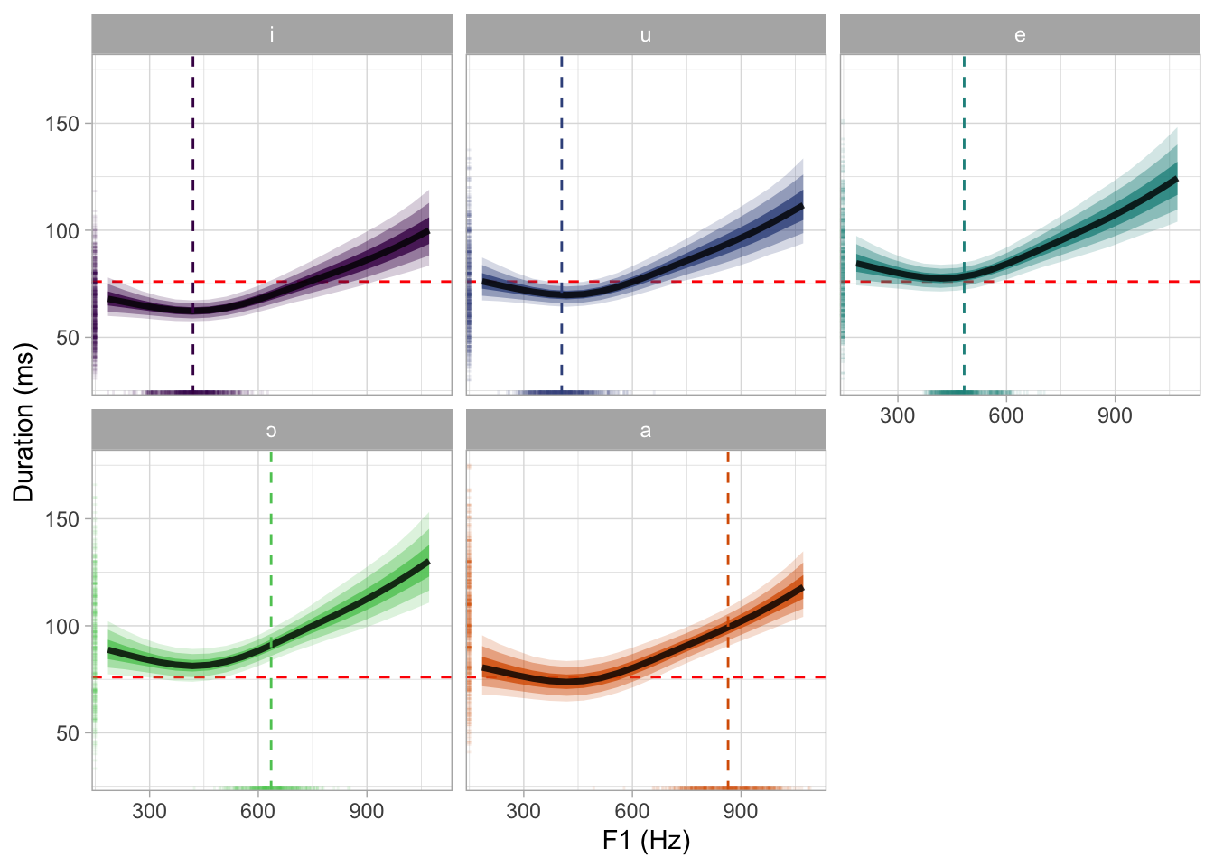

ggsave("img/bms1-pred-plot-ms-hz.png", width = 7, height = 5)

7 Non-linear modelling: mgcv F1 and F2

This is extra modelling of F1/F2 using mgcv. Does not feature in the publication and it’s unrelated to the research questions of the paper.

gam_2 <- bam(
  duration_logz ~
    vowel +
    s(f13_z, f23_z) +
    s(f13_z, f23_z, speaker, bs = "fs", m = 1),
  data = ita_egg
)

summary(gam_2)

Family: gaussian 
Link function: identity 

Formula:
duration_logz ~ vowel + s(f13_z, f23_z) + s(f13_z, f23_z, speaker, 
    bs = "fs", m = 1)

Parametric coefficients:
            Estimate Std. Error t value Pr(>|t|)    
(Intercept) -0.03176    0.18200  -0.175 0.861477    
vowele       0.43854    0.15991   2.742 0.006137 ** 
voweli      -0.31252    0.16553  -1.888 0.059128 .  
vowelo       0.38534    0.10901   3.535 0.000414 ***
vowelu      -0.11135    0.15542  -0.716 0.473775    
---
Signif. codes:  0 '***' 0.001 '**' 0.01 '*' 0.05 '.' 0.1 ' ' 1

Approximate significance of smooth terms:
                          edf Ref.df     F p-value    
s(f13_z,f23_z)          12.89  16.78 4.814  <2e-16 ***
s(f13_z,f23_z,speaker) 102.60 567.00 6.872  <2e-16 ***
---
Signif. codes:  0 '***' 0.001 '**' 0.01 '*' 0.05 '.' 0.1 ' ' 1

R-sq.(adj) =  0.708   Deviance explained = 71.9%
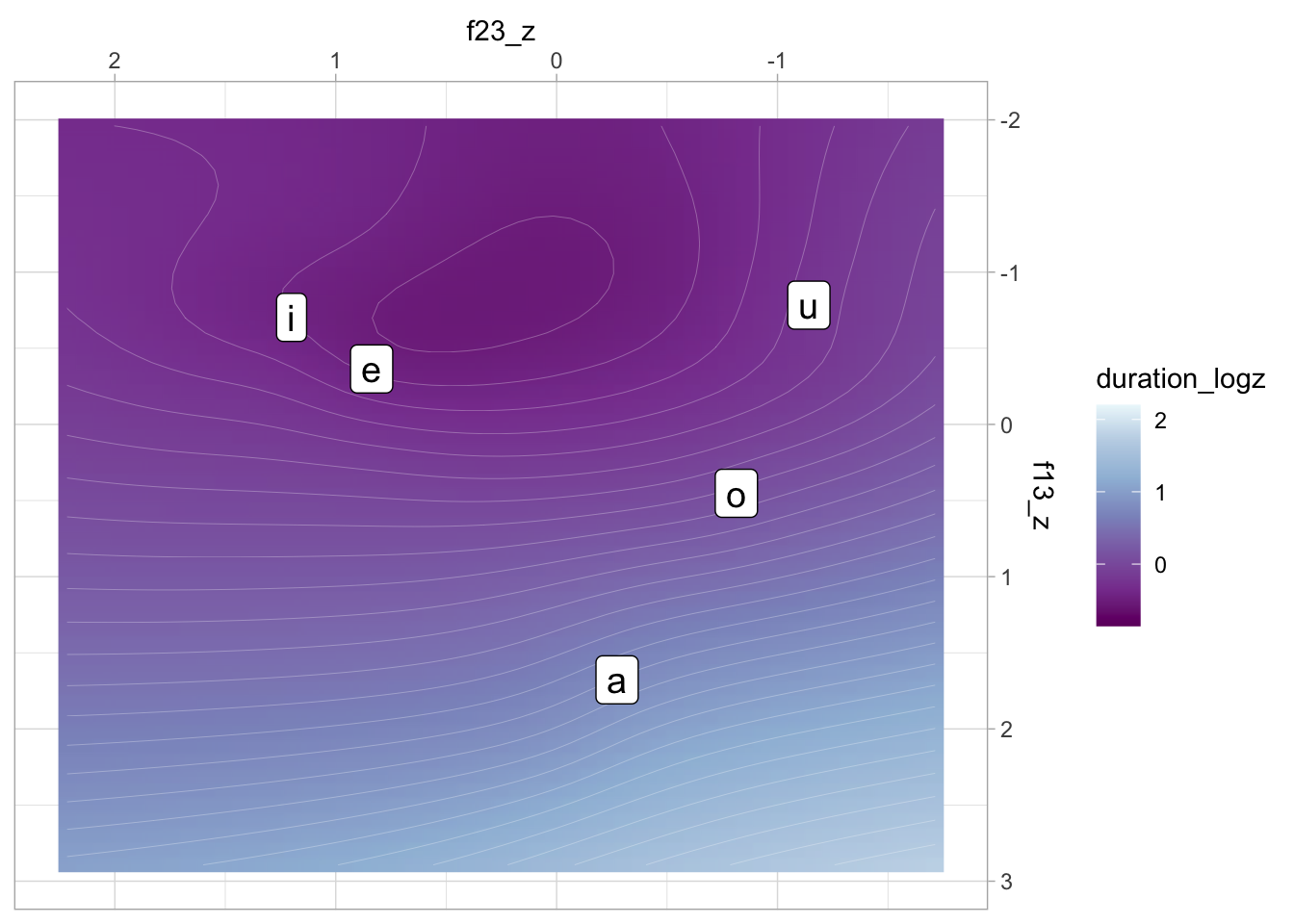
fREML = 2575.1  Scale est. = 0.29223   n = 3019

gam_2_preds <- predict_gam(gam_2, length_out = 50, exclude_terms = "s(f13_z,f23_z,speaker)")

vmeans <- ita_egg |>
  group_by(vowel) |>
  summarise(
    f13_z = mean(f13_z), f23_z = mean(f23_z)
  )

gam_2_preds |>
  ggplot(aes(f23_z, f13_z)) +
  geom_raster(aes(fill = duration_logz), interpolate = TRUE) +
  geom_contour(aes(z = duration_logz), bins = 40, colour = "white", linewidth = 0.05) +
  geom_label(data = vmeans, aes(label = vowel), size = 5) +
  scale_x_reverse(position = "top") +
  scale_y_reverse(position = "right") +
  scale_fill_distiller(palette = "BuPu")

Warning: Contour data has duplicated x, y coordinates.
ℹ 244494 duplicated rows have been dropped.