SQM tutorial - Week 5

Emotional valence of sense words

We will model data from Winter, 2016. Taste and smell words form an affectively loaded part of the English lexicon. DOI: 10.1080/23273798.2016.1193619. The study looked at the emotional valence of sense words in English, in the domains of taste and smell.

To download the file with the data right-click on the following link and download the file: senses_valence.csv. (Note that tutorial files are also linked in the Syllabus). Remember to save the file in data/ in the course project folder.

Create a new .Rmd file first, save it in code/ and name it tutorial-w05 (the extension .Rmd is added automatically!).

I leave to you creating title headings in your file as you please. Remember to to add knitr::opts_knit$set(root.dir = here::here()) in the setup chunk and to attach the tidyverse.

Let’s read the data. The original data also include words from other senses, so for this tutorial we will filter the data to include only smell and taste words.

senses_valence <- read_csv("data/senses_valence.csv") %>%
  filter(
    Modality %in% c("Smell", "Taste")
  )

Rows: 405 Columns: 3
── Column specification ────────────────────────────────────────────────────────
Delimiter: ","
chr (2): Word, Modality
dbl (1): Val

ℹ Use `spec()` to retrieve the full column specification for this data.
ℹ Specify the column types or set `show_col_types = FALSE` to quiet this message.

There are three columns:

• Word: the English word [categorical].

• Modality: Taste or Smell [categorical].

• Val: emotional valence [numeric, continuous]. The higher the number the more positive the valence.

Let’s quickly check the range of values in Val.

range(senses_valence$Val)

[1] 4.630476 6.436000

This is what the density plot of Val looks like.

senses_valence %>%
  ggplot(aes(Val)) +
  geom_density(fill = "gray", alpha = 0.5) +
  geom_rug()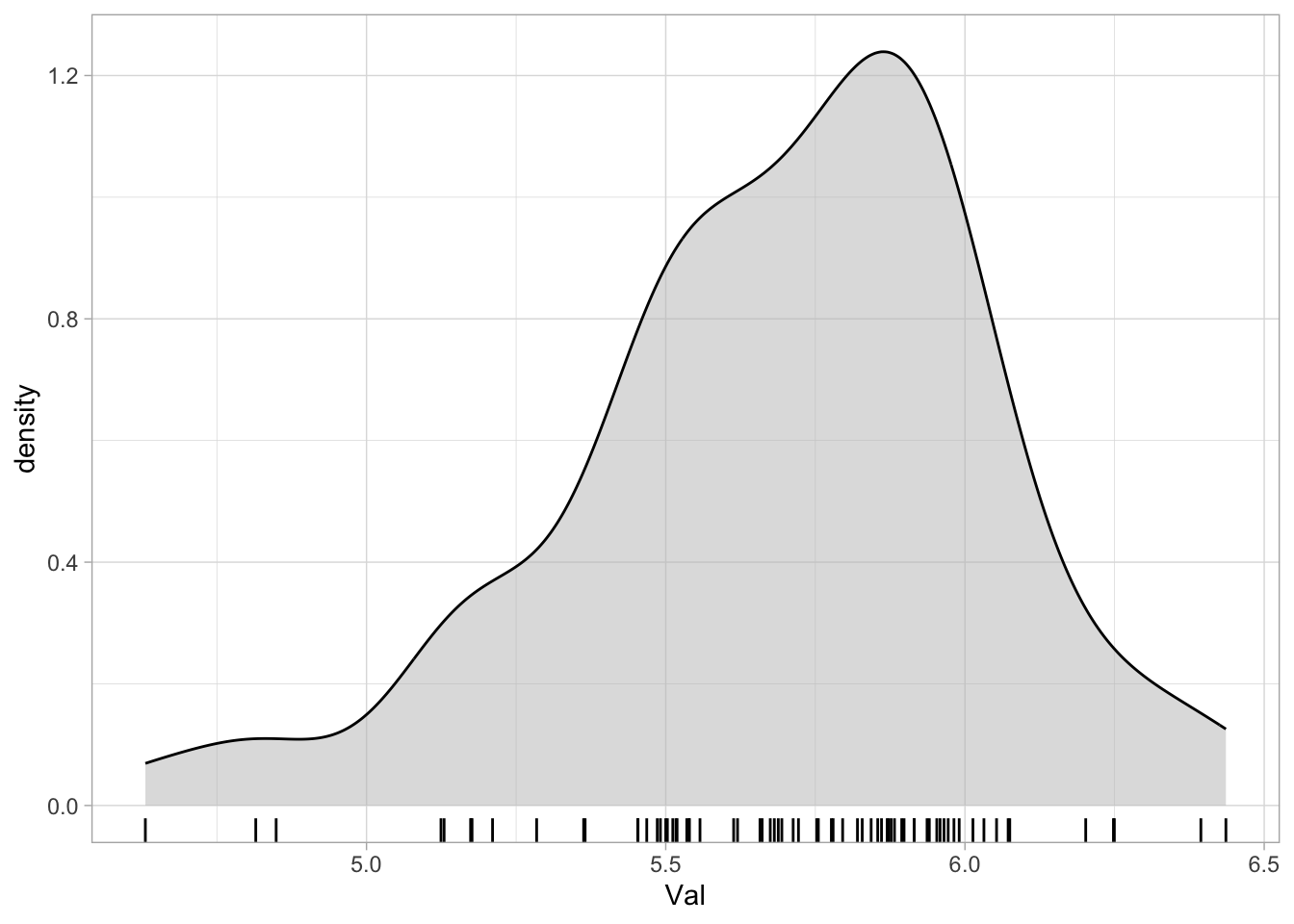

And if we separate by Modality (by using the fill parameter), we can see that the density of taste words is shifted towards higher values than that of smell words.

senses_valence %>%
  ggplot(aes(Val, fill = Modality)) +
  geom_density(alpha = 0.5) +
  geom_rug()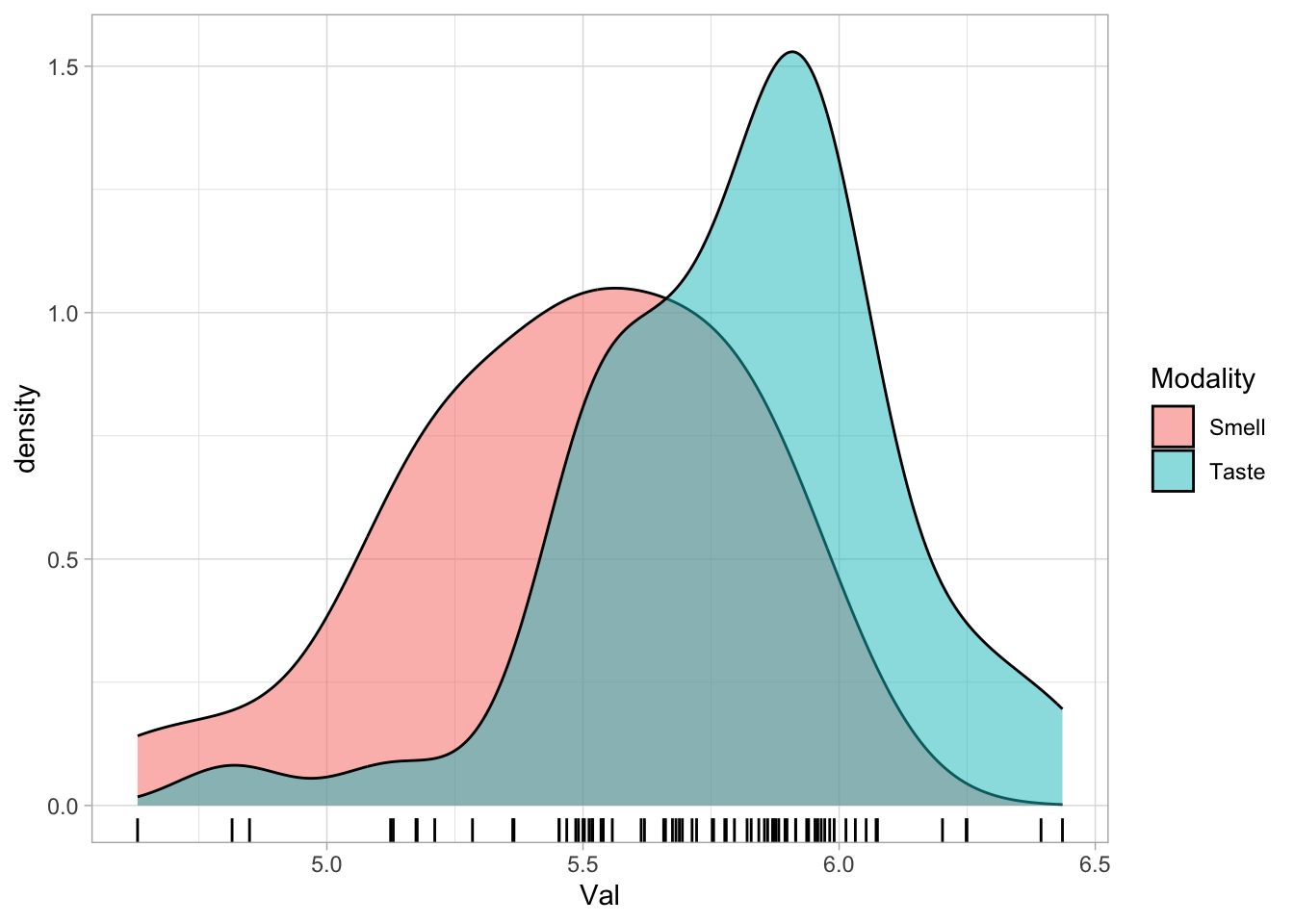

The plot thus suggests that, in this sample of 72 words, taste words are generally associated with a somewhat higher emotional valence than smell words.

Modelling emotional valence

Now that we got an overview of what the data looks like, let’s move onto modelling it with brm()!

Let’s assume, as we did with the VOT values, that the emotional valence values come from a Gaussian distribution.¹ In notation:

\[ \text{val} \sim Gaussian(\mu, \sigma) \]

Now, we want to estimate \(\mu\) so that we take into consideration whether the modality is “smell” or “taste”. In other words, we want to model valence as a function of modality, in R code Val ~ Modality.

Modality is a categorical variable (a chr character column in sense_valence) so it is coded using the default treatment coding system (this is done under the hood by R for you!). Since Modality has 2 levels, R will create for us a N-1 = 1 dummy variable (for illustration, we can imagine that it’s called modality_taste).

This is what the coding would look like:

	modality_taste
modality = smell	0
modality = taste	1

(R assigns the reference level, i.e., 0, to “smell”, because “s” comes before “t” in the alphabet.)

Now we allow \(\mu\) to vary depending on modality.

\[ \mu = \beta_0 + \beta_1 \cdot modality_{Taste} \]

Let’s unpack that. There’s a bit of algebra in what follows, so take your time if this is a bit out of your comfort zone. But it’s worth it—comfort with basic algebra will also help you become more comfortable working with linear models.

• \(\beta_0\) is the mean valence \(\mu\) when [modality = smell]. That’s because the variable \(modality_{Taste}\) takes on the value 0 when [modality = smell] (as we can see from the table above). Multiplying by 0 means that \(\beta_1\) vanishes from the equation, and all that’s left is \(\beta_0\).

\[ \begin{aligned} \mu &= \beta_0 + \beta_1 \cdot modality_{Taste}\\ \mu_{mod = smell} &= \beta_0 + \beta_1 \cdot 0 \\ \mu_{mod = smell} &= \beta_0 \\ \end{aligned} \]

• \(\beta_1\) is the difference in mean valence \(\mu\) between the mean valence when [modality = smell] and the mean valence when [modality = taste]. That’s because \(modality_{Taste}\) takes on the value 1 when [modality = taste], and multiplying \(\beta_1\) by 1 leaves it unchanged in the equation.

\[ \begin{aligned} \mu &= \beta_0 + \beta_1 \cdot modality_{Taste}\\ \mu_{mod = taste} &= \beta_0 + \beta_1 \cdot 1 \\ \mu_{mod = taste} &= \beta_0 + \beta_1 \\ \end{aligned} \]

• How do we know that \(\beta_1\) really represents the difference between the mean valence when [modality = smell] and the mean valence when [modality = taste]? Remember that \(\mu_{mod = smell} = \beta_0\), as we said in the first point above. We can substitute this into the equation from the last point, and then isolate \(\beta_1\) step by step as follows:

\[ \begin{aligned} \mu_{mod = taste} &= \beta_0 + \beta_1 \\ \mu_{mod = taste} &= \mu_{mod=smell} + \beta_1 \\ \mu_{mod = taste} - \mu_{mod=smell} &= \beta_1 \end{aligned} \]

So, \(\beta_1\) really is the difference between the means of these two levels of Modality.

Now we can define the probability distributions of \(\beta_0\) and \(\beta_1\).

\[ \beta_0 \sim Gaussian(\mu_0, \sigma_0) \]

\[ \beta_1 \sim Gaussian(\mu_1, \sigma_1) \]

And the usual for \(\sigma\).

\[ \sigma \sim TruncGaussian(\mu_2, \sigma_2) \]

All together, we need to estimate the following parameters: \(\mu_0, \sigma_0, \mu_1, \sigma_1, \mu_2, \sigma_2\).

Run the model

Now we know what the model will do, we can run it.

Before that though, create a folder called cache/ in the data/ folder of the RStudio project of the course. We will use this folder to save the output of model fitting so that you don’t have to refit the model every time. (This is useful because as models get more and more complex, they can take quite a while to fit.)

After you have created the folder, run the following code.

val_bm <- brm(
  Val ~ Modality,
  family = gaussian(),
  data = senses_valence,
  backend = "cmdstanr",
  # Save model output to file
  file = "data/cache/val_bm"
)

The model will be fitted and saved in data/cache/ with the file name val_bm.rds. If you now re-run the same code again, you will notice that brm() does not fit the model again, but rather reads it from the file (no output is shown, but trust me, it works! Check the contents of data/cache/ to see for yourself.).

Model interpretation

Let’s inspect the model summary.

summary(val_bm)

 Family: gaussian 
  Links: mu = identity; sigma = identity 
Formula: Val ~ Modality 
   Data: senses_valence (Number of observations: 72) 
  Draws: 4 chains, each with iter = 2000; warmup = 1000; thin = 1;
         total post-warmup draws = 4000

Population-Level Effects: 
              Estimate Est.Error l-95% CI u-95% CI Rhat Bulk_ESS Tail_ESS
Intercept         5.47      0.06     5.35     5.59 1.00     3800     3149
ModalityTaste     0.34      0.08     0.18     0.50 1.00     3866     2984

Family Specific Parameters: 
      Estimate Est.Error l-95% CI u-95% CI Rhat Bulk_ESS Tail_ESS
sigma     0.32      0.03     0.27     0.38 1.00     3136     2573

Draws were sampled using sample(hmc). For each parameter, Bulk_ESS
and Tail_ESS are effective sample size measures, and Rhat is the potential
scale reduction factor on split chains (at convergence, Rhat = 1).

Look at the Population-Level Effects part of the summary.

Population-Level Effects: 
              Estimate Est.Error l-95% CI u-95% CI Rhat Bulk_ESS Tail_ESS
Intercept         5.47      0.06     5.35     5.59 1.00     3800     3149
ModalityTaste     0.34      0.08     0.18     0.50 1.00     3866     2984

We get two “effects” or coefficients:

• Intercept: this is our \(\beta_0\).

• ModalityTaste: this is our \(\beta_1\).

Each coefficient has an Estimate and an Est.Error (estimate error). As we have seen last week, these are the mean and SD of the probability distribution of the coefficients.

In notation:

\[ \beta_0 = Gaussian(5.47, 0.06) \]

\[ \beta_1 = Gaussian(0.34, 0.08) \]

This means that:

• The probability distribution of the mean valence when [modality = smell] is a Gaussian distribution with mean = 5.47 and SD = 0.06.

• The probability distribution of the difference between the mean valence of [modality = taste] and that of [modality = smell] is a Gaussian distribution with mean = 0.34 and SD = 0.08.

Now look at the Credible Intervals (CrIs, or CI in the model summary) of the coefficients. Based on their CrIs, we can say that:

• We can be 95% confident that (or, there is 95% probability that), based on the data and the model, the mean emotional valence of smell words is between 5.35 and 5.59.

• There is a 95% probability that the difference in mean emotional valence between taste and smell words is between 0.18 and 0.5. In other words, the emotional valence increases by 0.18 to 0.5 in taste words relative to smell words.

Plotting probability distributions

They say a plot is better than a thousand words, so why don’t we plot the probability distributions of the Intercept (\(\beta_0\)) and ModalityTaste (\(\beta_1\)) coefficients?

Before we do, just a quick terminological clarification.

Posterior probability distributions

Posterior probability distribution

The probability distributions of model coefficients obtained through model fitting with brm() are called posterior probability distributions.

We will see why they are called that and what prior probability distributions are, but for the time being, just remember that when we talk about posterior probability distributions we are talking about the probability distributions of the model coefficients.

So, how do we plot posterior probability distributions?

There are different methods, each of which has its own advantages and disadvantages. Some methods require extra packages, while others work with the packages you already know of.

To simply things, we will use a method that works out of the box with just ggplot2. The first step to plot posterior distributions is to extract the values to be plotted from the model output.

Posterior draws

Which values, you might ask? The coefficient values obtained with the MCMC draws. (Remember we talked about Markov Chain Monte Carlo iterations last week?). In order to estimate the coefficients, brm() runs a number of MCMC iterations and at each iteration a value for each coefficient in the model is proposed (this is a simplification, if you want to know more about the inner working of MCMCs, check the Statistical (Re)Thinking book).

At the end, what you get is a list of values for each coefficient in the model. These are called the posterior draws. The probability distribution of the posterior draws of a coefficient is the posterior probability distribution of that coefficient.

And, if you take the mean and standard deviation of the posterior draws of a coefficient, you get the Estimate and Est.Error values in the model output!

You can easily extract the posterior draws of all the model’s coefficients with the as_draws_df() function from the brms package.

val_bm_draws <- as_draws_df(val_bm)
val_bm_draws

Check the first three columns of the tibble (don’t worry about the other columns for now—those are technical things that are important for brms, but not so important for us). The first three columns are our \(\beta_0\), \(\beta_1\) and \(\sigma\) from the model formulae above!

• b_Intercept: \(\beta_0\).

• b_ModalityTaste: \(\beta_1\).

• sigma: \(\sigma\).

(Why is there a b at the beginning of b_Intercept and b_ModalityTaste? Well, “b” is for “beta”, and it’s brms’s way of telling us what kind of coefficient we’re working with.)

Fantastic! Now that we have the posterior draws as a nice tibble, we can use geom_density() from ggplot2 to plot the probability density, a.k.a., the posterior probability distribution, for each coefficient.

Plotting posteriors

Let’s start with the posterior probability, or posterior for short, of b_Intercept.

val_bm_draws %>%
  ggplot(aes(b_Intercept)) +
  geom_density(fill = "gray", alpha = 0.5) +
  labs(
    title = "Posterior probability distribution of Intercept"
  )

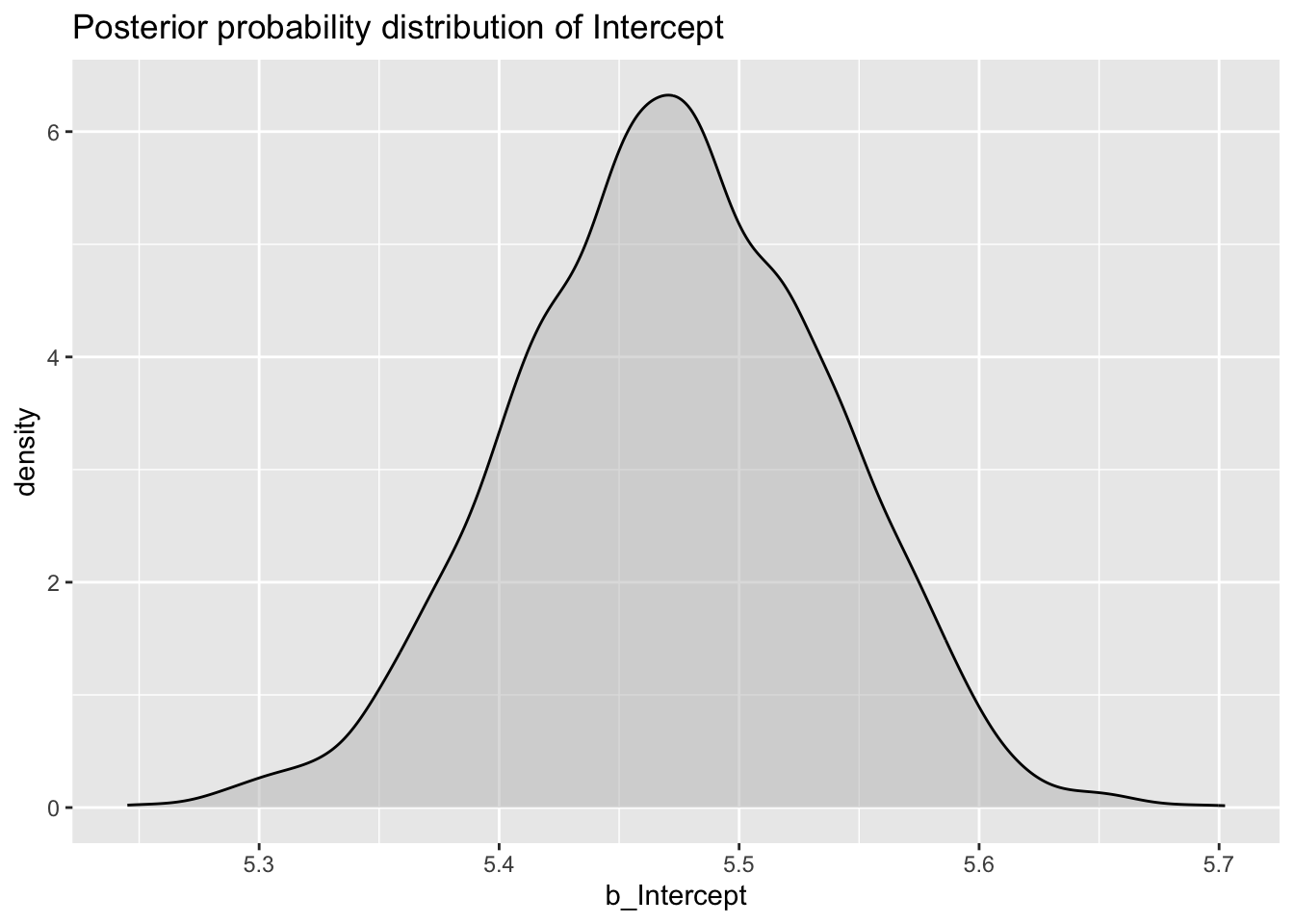
Nice, huh?

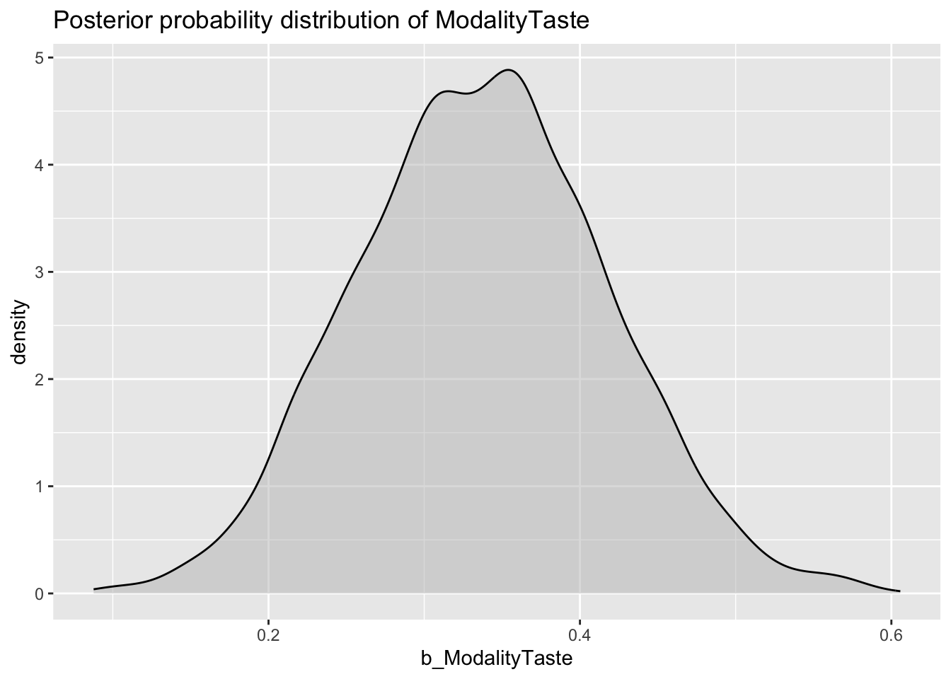
Now with b_ModalityTaste.

val_bm_draws %>%
  ggplot(aes(b_ModalityTaste)) +
  geom_density(fill = "gray", alpha = 0.5) +
  labs(
    title = "Posterior probability distribution of ModalityTaste"
  )

If you feel like it, go ahead and plot the posterior distribution of sigma as well.

Plotting conditional probability distributions

This is all great, but what if you wanted to know the probability distribution of mean emotional valence in either smell or taste words? So far, we only know the probability distribution of mean valence for smell words (\(\beta_0\)), and how that valence is changed for taste words (\(\beta_1\)). We don’t yet know the probability distribution of mean emotional valence for taste words. How do we find that distribution?

This is where conditional posterior probability distributions (or conditional probabilities for short) come in!

They are posterior probability distributions like the ones we have plotted above, but they are conditional on specific values of each predictor in the model.

In the val_bm model we had only included one predictor (we will see how to include more in the coming weeks): Modality, which has two levels Smell and Taste.

How do we obtain the conditional probabilities of emotional valence for smell and taste words respectively?

The formula of \(\mu\) above can help us solve the mystery.

\[ \mu = \beta_0 + \beta_1 \cdot modality_{Taste} \]

The conditional probability of mean emotional valence in smell words is just \(\beta_0\). Why? Remember that when [modality = smell], \(modality_{Taste}\) is 0, so:

\[ \beta_0 + \beta_1 \cdot 0 = \beta_0 \]

In other words, the conditional probability of mean emotional valence in smell words is equal to the posterior probability of b_Intercept. This is so because Modality is coded using the treatment coding system (nothing mysterious here).

But what about taste words? Here’s where we need to do some more maths/data processing.

When [modality = taste], \(modality_{Taste}\) is 1, so:

\[ \beta_0 + \beta_1 \cdot 1 = \beta_0 + \beta_1 \]

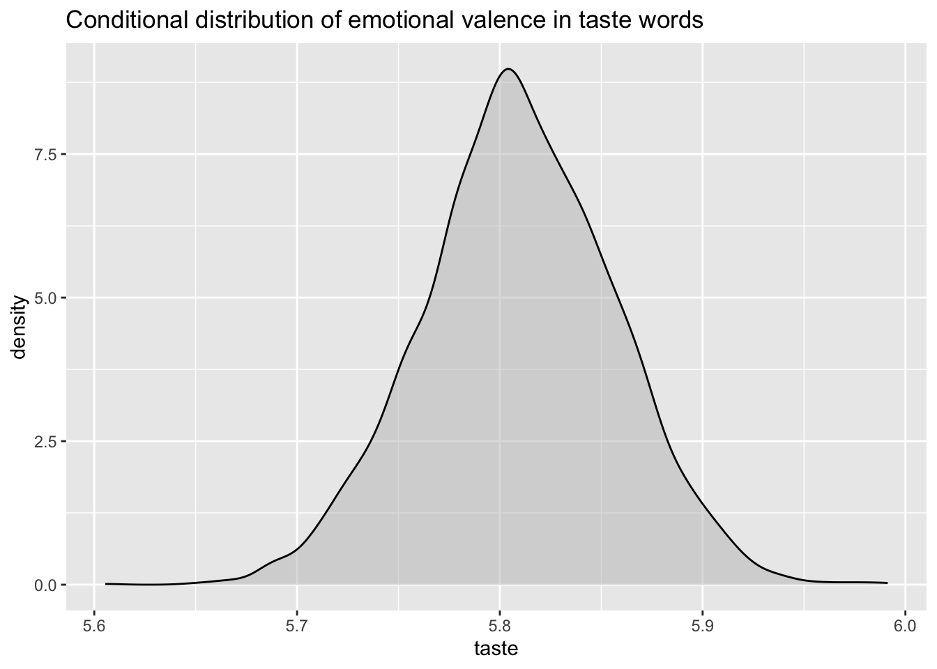
So to get the conditional posterior probability of mean emotional valence for taste words, we need to sum the posterior draws of b_Intercept (\(\beta_0\)) and b_ModalityTaste (\(\beta_1\)): \(\beta_0 + \beta_1\).

It couldn’t be easier than using the mutate() function from dplyr. Remember that mutate() creates a new column (here, called taste) based on the values of other columns. Here, we’re just adding together the values in b_Intercept and those in b_ModalityTaste (a.k.a., the posterior draws for each of those coefficients).

val_bm_draws <- val_bm_draws %>%
  mutate(
    taste = b_Intercept + b_ModalityTaste
  )

Now, we can just plot the probability density of taste to get the conditional posterior probability distribution of mean emotional valence for taste words.

val_bm_draws %>%
  ggplot(aes(taste)) +
  geom_density(fill = "gray", alpha = 0.5) +
  labs(
    title = "Conditional distribution of emotional valence in taste words"
  )

What if you want to show both the conditional probability of emotional valence in smell and taste words? Easy!²

val_bm_draws %>%
  ggplot() +
  geom_density(aes(b_Intercept), fill = "red", alpha = 0.5) +
  geom_density(aes(taste), fill = "blue", alpha = 0.5) +
  labs(
    title = "Conditional distributions of mean emotional valence in smell vs taste words"
  )

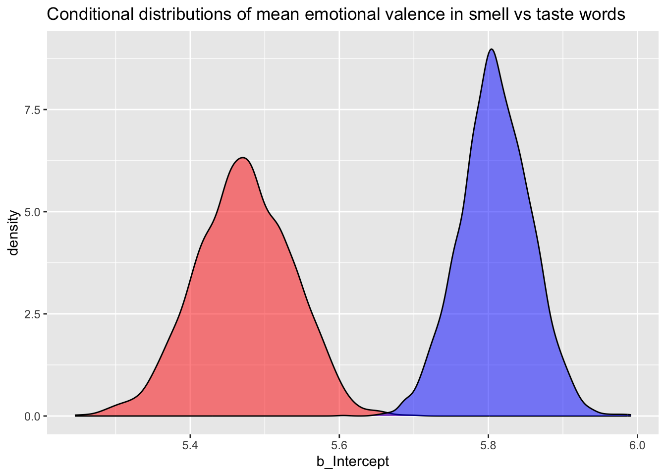
Based on this plot, we can say that the model suggests a different mean emotional valence for smell vs. taste words, and that taste words (blue) have a more positive emotional valence than smell words (red).

To reiterate from above, based on the 95% CrI of b_ModalityTaste, there is a 95% probability that the mean emotional valence of taste words is 0.18 to 0.5 greater than that of smell words.

You might ask now: Is this difference relevant? Unfortunately, statistics cannot help you to answer that question (remember, we imbue numbers with meaning). Only conceptual theories of lexical emotional valence can (or cannot)!

Morphological processing and reaction times

So far, we’ve seen how to work with treatment-coded variables with only two levels. In this last section, we’ll take a look at how to use dummy coding for a variable with three levels.

You might remember the shallow.csv data we used in Week 2, from Song et al. 2020. Second language users exhibit shallow morphological processing. DOI: 10.1017/S0272263120000170.

The study compared results of English L1 vs L2 participants and of left- vs right-branching words, but for this tutorial we will only be looking at the L1 and left-branching data.

The data file also contains data from the filler items, which we filter out.

shallow <- read_csv("data/shallow.csv") %>%
  filter(
    Group == "L1",
    Branching == "Left",
    Critical_Filler == "Critical",
    RT > 0
  )

Rows: 6500 Columns: 11
── Column specification ────────────────────────────────────────────────────────
Delimiter: ","
chr (8): Group, ID, List, Target, Critical_Filler, Word_Nonword, Relation_ty...
dbl (3): ACC, RT, logRT

ℹ Use `spec()` to retrieve the full column specification for this data.
ℹ Specify the column types or set `show_col_types = FALSE` to quiet this message.

shallow

The study consisted of a lexical decision task in which participants where first shown a prime, followed by a target word for which they had to indicate whether it was a real word or a nonce word.

The prime word belonged to one of three possible groups (Releation_type in the data) each of which refers to the morphological relation of the prime and the target word:

• Unrelated: for example, prolong (assuming unkindness as target, [[un-kind]-ness]).

• Constituent: unkind.

• NonConstituent: kindness.

The expectation is that lexical decision for native English participants should be facilitated in the Constituent condition, but not in the Unrelated and NonConstituent conditions (if you are curious as to why that is the expectation, I refer you to the paper).

Let’s interpret that as:

The Constituent condition should elicit shorter reaction times than the other two conditions.

Before moving on, let’s visualise the reaction times (RT) values which are in milliseconds.

shallow %>%
  ggplot(aes(RT)) +
  geom_density() +
  geom_rug()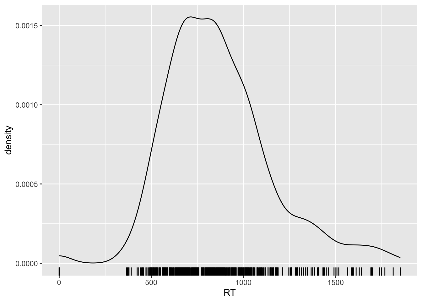

You will notice that RT can only be positive: reaction time is a numeric continuous variable, bounded to positive numbers only!

Remember how we talked above about choosing an appropriate distribution to model your data? Variables that are bounded to positive numbers are known not to be distributed according to a Gaussian distribution. Each case might be a bit different, but when a variable is bounded (e.g., by zero), it is very safe to assume that the values of the variable do not follow a Gaussian distribution.³

Log-transformation

But we have a trick in our pocket: just calculate the logarithm of the values and they will conform to a Gaussian distribution! This is a common trick in psycholinguistics for modelling reaction time data. You can calculate the logarithm (or log) of a number in R using the log() function. Calculating the logs of a variable is known as a log-transformation.

I will illustrate what this looks like with the first five values of RT in shallow.

RT <- c(603, 739, 370, 821, 1035)
RT

[1]  603  739  370  821 1035

log(RT)

[1] 6.401917 6.605298 5.913503 6.710523 6.942157

So the log of 603 is 6.4, the log of 739 is 6.6 and so on.

The shallow data table already has a column with the log-transformed RTs: logRT. So let’s plot that now.

shallow %>%
  ggplot(aes(logRT)) +
  geom_density() +
  geom_rug()

Warning: Removed 4 rows containing non-finite values (`stat_density()`).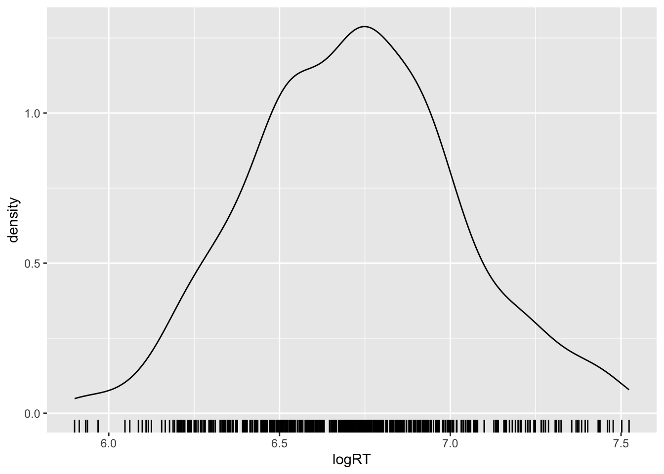

Warning: it is usually not possible to rely on the shape of the probability density to determine if the probability is Gaussian or not! Rather, ask yourself the following question: are the values bounded to positive numbers only? If the answer is “yes”, then the variable is not Gaussian and you know you can log-transform it.

Log-normal distribution

Variables that are Gaussian (normal) when they are log-transformed follow the log-normal distribution.

Now let’s look at a violin and strip plot with Relation_type on the x-axis and logRT on the y-axis.

shallow %>%
  ggplot(aes(Relation_type, logRT, fill = Relation_type)) +
  geom_violin() +
  geom_jitter(width = 0.1, alpha = 0.2)

Warning: Removed 4 rows containing non-finite values (`stat_ydensity()`).

Warning: Removed 4 rows containing missing values (`geom_point()`).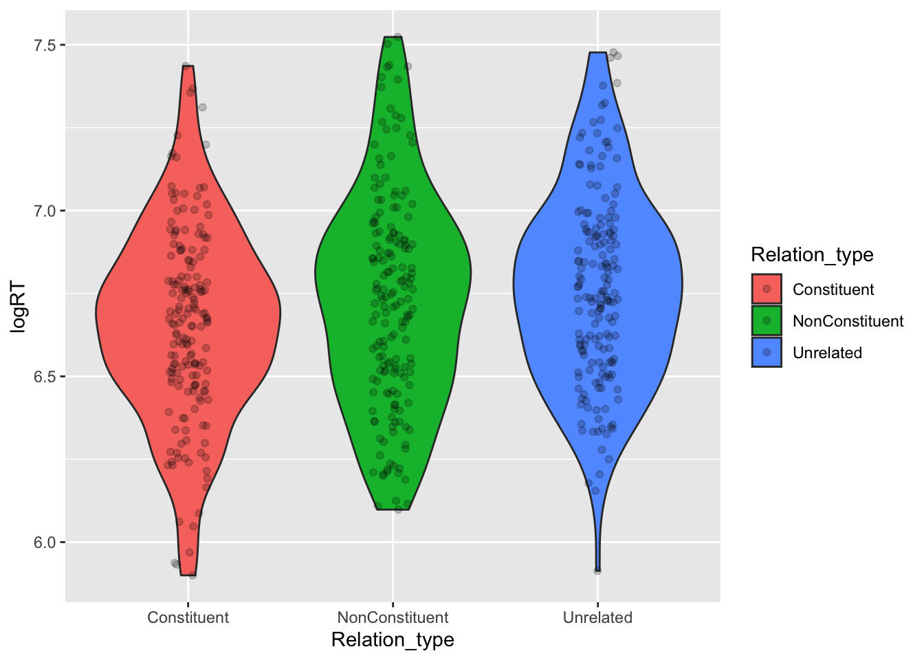

Based on this, we can see that the bulk of the distribution (the place where the violin is wider) falls somewhat lower on the log-RT scale for the Constituent condition relative to the other conditions.

Ordering levels of a categorical predictor

By default, the levels in Relation_type follow the order: Constituent, NonConstituent, Unrelated (this is the default alphabetical order).

There is nothing bad with this per se, but maybe we can reorder them so that they are in this order: Unrelated, NonConstituent, Constituent.

This might make a bit more sense from a conceptual point of view (you can think of the unrelated condition as the “baseline” condition).

To order levels in R, we can use a factor variable/column.

shallow <- shallow %>%
  mutate(
    Relation_type = factor(Relation_type, levels = c("Unrelated", "NonConstituent", "Constituent"))
  )

This overwrites the Relation_type column so that the levels are in the specified order. You can check this in the Environment tab: click on the blue arrow next to shallow to see the column list and now Relation_type is a Factor column with 3 levels.

Model RTs by relation type

Now it’s your turn! With the following guidance, go ahead and run a model with brm() to investigate the effect of relation type on log-RT. Inspect the model summary and plot the posterior probabilities.

Relation_type is a categorical variable with three levels, so here’s what treatment coding looks like (there will be N-1 = 3-1 = 2 dummy variables).

	relation_ncons	relation_cons
relation = unrelated	0	0
relation = non-constituent	1	0
relation = constituent	0	1

Here are a few formulae that describe in mathematical notation the model that we’ll need to fit. Try to go through them and unpack them based on what you’ve learned above and in the lecture.

\[ \begin{aligned} \text{logRT} &\sim Gaussian(\mu, \sigma) \\ \mu &= \beta_0 + \beta_1 \cdot relation_{ncons} + \beta_2 \cdot relation_{cons} \\ \beta_0 &\sim Gaussian(\mu_0, \sigma_0)\\ \beta_1 &\sim Gaussian(\mu_1, \sigma_1)\\ \beta_2 &\sim Gaussian(\mu_2, \sigma_2)\\ \sigma &\sim TruncGaussian(\mu_3, \sigma_3) \end{aligned} \]

Focus especially on \(\beta_0\), \(\beta_1\) and \(\beta_2\). What do they correspond to?

Fit the model with brm(). What does the R formula for this model look like?

Check the model summary. What can you say based on the estimates and the CrIs?

Plot the posterior probability distributions of \(\beta_0\), \(\beta_1\) and \(\beta_2\) and the conditional probability distributions of mean log-RTs for each relation type.

A hint for the conditional probability distributions: to plot these you need to sum the posterior draws of the beta coefficients depending on the level of relation type. Use the formula of \(\mu\) to guide you: the process is the same as with the emotional valence data above, but now there are 3 levels instead of two.

Summary

Treatment coding

• Categorical predictors need to be coded as numbers.
• N-1 dummy variables, where N is number of levels in the predictor.
• Level ordering is alphabetical but you can specify your own.
• NOTE: you don’t have to apply treatment coding yourself! It’s done under the hood by R.

Interpreting coefficients

• The Intercept \(\beta_0\) is the mean of the reference level.
• The other \(\beta\)’s are the difference of the other levels relative to the reference level.

Conditional posterior probability distributions

• To calculate the conditional posterior probability distributions (conditional probabilities for short) you need to extract the draws of the model with as_draws_df().

Log-normal distribution

• Continuous variables that are Gaussian when transformed to logs follow the log-normal distribution.

• You can fit a Gaussian model to log-transformed values if the variable is log-normal.

Footnotes

1. Note that, in real-life research contexts, you should decide which distribution to use for different outcome variables by drawing on previous research that has assessed the possible distribution families for those variables, on domain-specific expertise or common-sense. You will see that in most cases with linguistic phenomena we know very little about the nature of the variables we work with, hence it can be difficult to know which family of distributions to use.

2. The following code is a bit of a hack. There is a better way to do this using pivot_longer() from the tidyr package. We will learn how to use this and other functions from that package later in the course.

3. In fact, we have assumed above that emotional valence is distributed according to a Gaussian distribution, and we got lucky that this assumption in principle holds for the values in the data sample, because emotional valence as measured in the study is actually bounded between 1 and 8. In most cases you won’t be lucky, so always carefully think about the nature of your variables. Again, only conceptual theories of the phenomena you are investigating will be able to help.