library(tidyverse)

pupil_width <- read_csv("https://raw.githubusercontent.com/uoelel/qml-data/refs/heads/main/data/mclaughlin2023/pupil-width.csv")

pupil_widthObtaining expected values from the posterior predictive distribution in brms models
Regression models
Bayesian
brms
Statistics
Once you fit a Bayesian regression model with brms::brm(), virtually all subsequent operations are based on the model’s MCMC draws. Once estimand of interest, that is derived from the MCMC draws, are the expected values of the posterior predictive distribution.
There are several ways of calculating/extracting the expected values. This post is intended to showcase these methods. Prior familiarity with Bayesian regression modelling and the brms package (Bürkner 2017) are necessary.
1 Manual computation from the draws
The most basic approach is to extract the MCMC draws from the model and compute the expected values from them. The following model uses data from McLaughlin et al. (2022), a study of how pupil width covaries with lexical neighbourhood density. Let’s read the data.
Our variables of interest are pupil_max, the maximum pupil size within trial, scaled within trial and participant, and Condition, either Dense or Sparse neighbourhood. We can now fit a BRM.
library(brms)

pupil_bm <- brm(
  pupil_max ~ Condition,
  family = gaussian,
  data = pupil_width,
  cores = 4, seed = 732, file = "posts/2025-11-08-expected-predictions/pupil_bm"
)

summary(pupil_bm, prob = 0.8)
Family: gaussian
Links: mu = identity
Formula: pupil_max ~ Condition
Data: pupil_width (Number of observations: 10588)
Draws: 4 chains, each with iter = 2000; warmup = 1000; thin = 1;
total post-warmup draws = 4000
Regression Coefficients:
Estimate Est.Error l-80% CI u-80% CI Rhat Bulk_ESS Tail_ESS
Intercept 1.02 0.01 1.00 1.03 1.00 3772 3092
ConditionSparse -0.01 0.01 -0.03 0.01 1.00 3747 3033
Further Distributional Parameters:
Estimate Est.Error l-80% CI u-80% CI Rhat Bulk_ESS Tail_ESS
sigma 0.75 0.01 0.74 0.75 1.00 4720 2723
Draws were sampled using sampling(NUTS). For each parameter, Bulk_ESS
and Tail_ESS are effective sample size measures, and Rhat is the potential
scale reduction factor on split chains (at convergence, Rhat = 1).We can calculate the expected values for the dense and sparse neighbourhoods by transforming the draws, obtained with as_draws_df() from the posterior package.
library(posterior)

pupil_draws <- as_draws_df(pupil_bm) |>
  mutate(
    dense = b_Intercept,
    sparse = b_Intercept + b_ConditionSparse
  )

head(pupil_draws)
You can then summarise and plot as with any type of data. Summarising can be done either manually with mutate() or with the summarise_draws() from the posterior package.
pupil_draws |>
  select(dense:sparse) |>
  summarise_draws() |>
  # Optional: show only 2 digits
  mutate(across(where(is.numeric), ~round(.x, 2)))
Warning: Dropping 'draws_df' class as required metadata was removed.For plotting the expected values with ggplot2, it is convenient to pivot the tibble.
pupil_draws_long <- pupil_draws |>
  select(.chain, .iteration, .draw, dense, sparse) |>
  pivot_longer(dense:sparse, names_to = "Condition", values_to = "epred")
Warning: Dropping 'draws_df' class as required metadata was removed.head(pupil_draws_long)We can use the stat_halfeye() function from the ggdist package.
library(ggdist)

pupil_draws_long |>
  ggplot(aes(epred, Condition)) +
  stat_halfeye()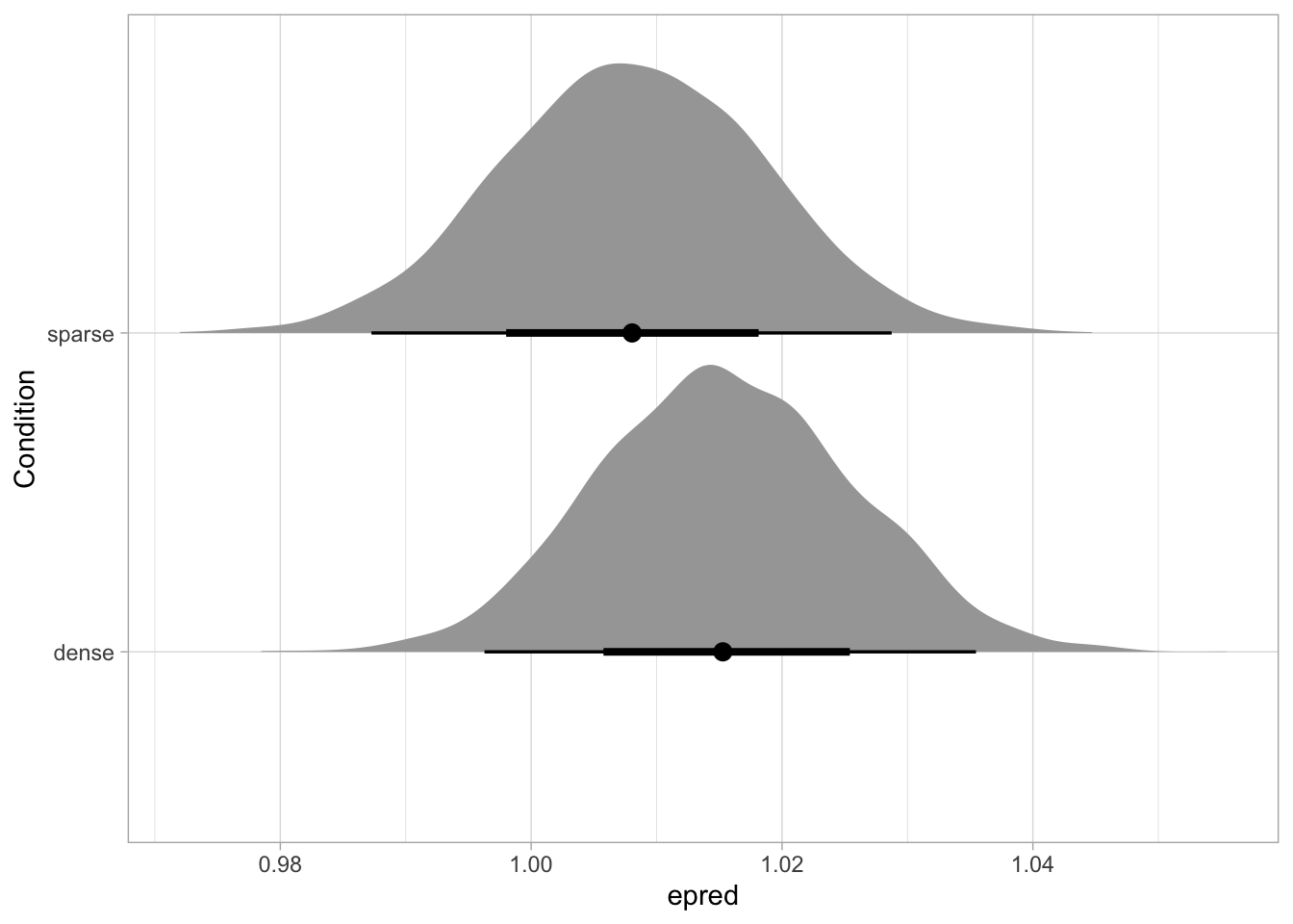
2 Plotting with conditional_effects()
Plotting the expected values can also be done with conditional_effects() from the brms package, which plots error bars with a central measure (by default, 95% CrI and the median). The function uses the posterior_epred method by default, which is the one that returns expected values (set explicitly in the code below for clarity).
conditional_effects(pupil_bm, method = "posterior_epred")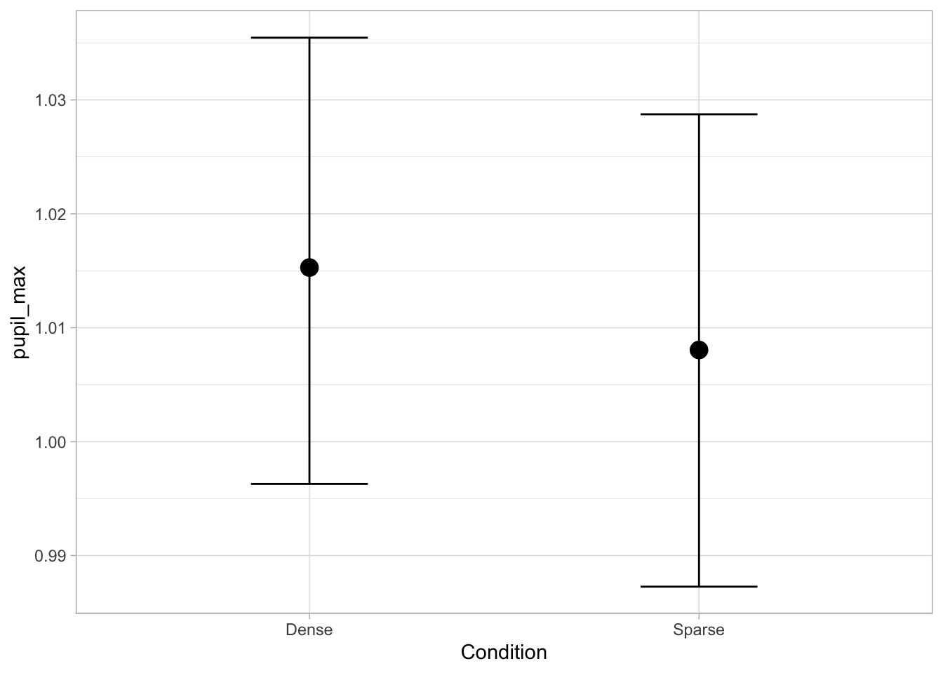
3 Computation with tidybayes
An alternative to manual computation is to use the epred_draws() from the tidybayes package. The function requires the user to input a “prediction grid” as newdata. For each row in the prediction grid, the expected value for each of the draws will be calculated. The returned tibble is in the “longer” format (like pupil_draws_long).
library(tidybayes)

pred_grid <- tibble(
  Condition = c("Dense", "Sparse")
)

pupil_epred <- epred_draws(
  pupil_bm,
  newdata = pred_grid
)

head(pupil_epred)
Using tidybayes::epred_draws() is convenient when the model has one or more numeric predictors. For example, let’s model data from Tucker et al. (2019). The data contains reactions times from an auditory lexical decision task in English. We can estimate the covariation between RTs, phone Levenshtein distance (higher values indicate the word is more unique compared to other words, PhonLev) and lexical status (real or non-real word, IsWord).
mald <- readRDS("data/tucker2019/mald_1_1.rds")

mald
Let’s model RTs with a log-normal regression.
mald_bm <- brm(
  RT ~ IsWord * PhonLev,
  family = lognormal,
  data = mald,
  cores = 4, seed = 732, file = "posts/2025-11-08-expected-predictions/mald_bm"
)

summary(mald_bm, prob = 0.8)
Family: lognormal
Links: mu = identity
Formula: RT ~ IsWord * PhonLev
Data: mald (Number of observations: 5000)
Draws: 4 chains, each with iter = 2000; warmup = 1000; thin = 1;
total post-warmup draws = 4000
Regression Coefficients:
Estimate Est.Error l-80% CI u-80% CI Rhat Bulk_ESS Tail_ESS
Intercept 6.52 0.03 6.48 6.56 1.00 1853 2265
IsWordFALSE 0.23 0.04 0.18 0.28 1.01 1269 1596
PhonLev 0.04 0.00 0.04 0.05 1.00 1849 2177
IsWordFALSE:PhonLev -0.02 0.01 -0.02 -0.01 1.01 1273 1631
Further Distributional Parameters:
Estimate Est.Error l-80% CI u-80% CI Rhat Bulk_ESS Tail_ESS
sigma 0.27 0.00 0.27 0.27 1.00 2445 1980
Draws were sampled using sampling(NUTS). For each parameter, Bulk_ESS
and Tail_ESS are effective sample size measures, and Rhat is the potential
scale reduction factor on split chains (at convergence, Rhat = 1).Using the draws from as_draws_df() would require calculating expected prediction manually for a range of values of PhonLev. Instead, we can use epred_draws() by specifying a sequence of values with seq() when creating the prediction grid with expand_grid() from the tidyr package.
pred_grid <- expand_grid(
  IsWord = c("FALSE", "TRUE"),
  PhonLev = seq(min(mald$PhonLev), max(mald$PhonLev), by = 0.1)
)

mald_epred <- epred_draws(mald_bm, newdata = pred_grid)

head(mald_epred)
We can plot the expected values with geom_line() and geom_ribbon().
mald_epred_summary <- mald_epred |>
  group_by(IsWord, PhonLev) |>
  summarise(
    mean = mean(.epred),
    lo = quantile2(.epred, 0.025),
    hi = quantile2(.epred, 0.975),
    .groups = "drop"
  )

mald_epred_summary |>
  ggplot(aes(PhonLev)) +
  geom_ribbon(aes(ymin = lo, ymax = hi, group = IsWord), alpha = 0.25) +
  geom_line(aes(y = mean, colour = IsWord)) +
  ylab("RT (ms)")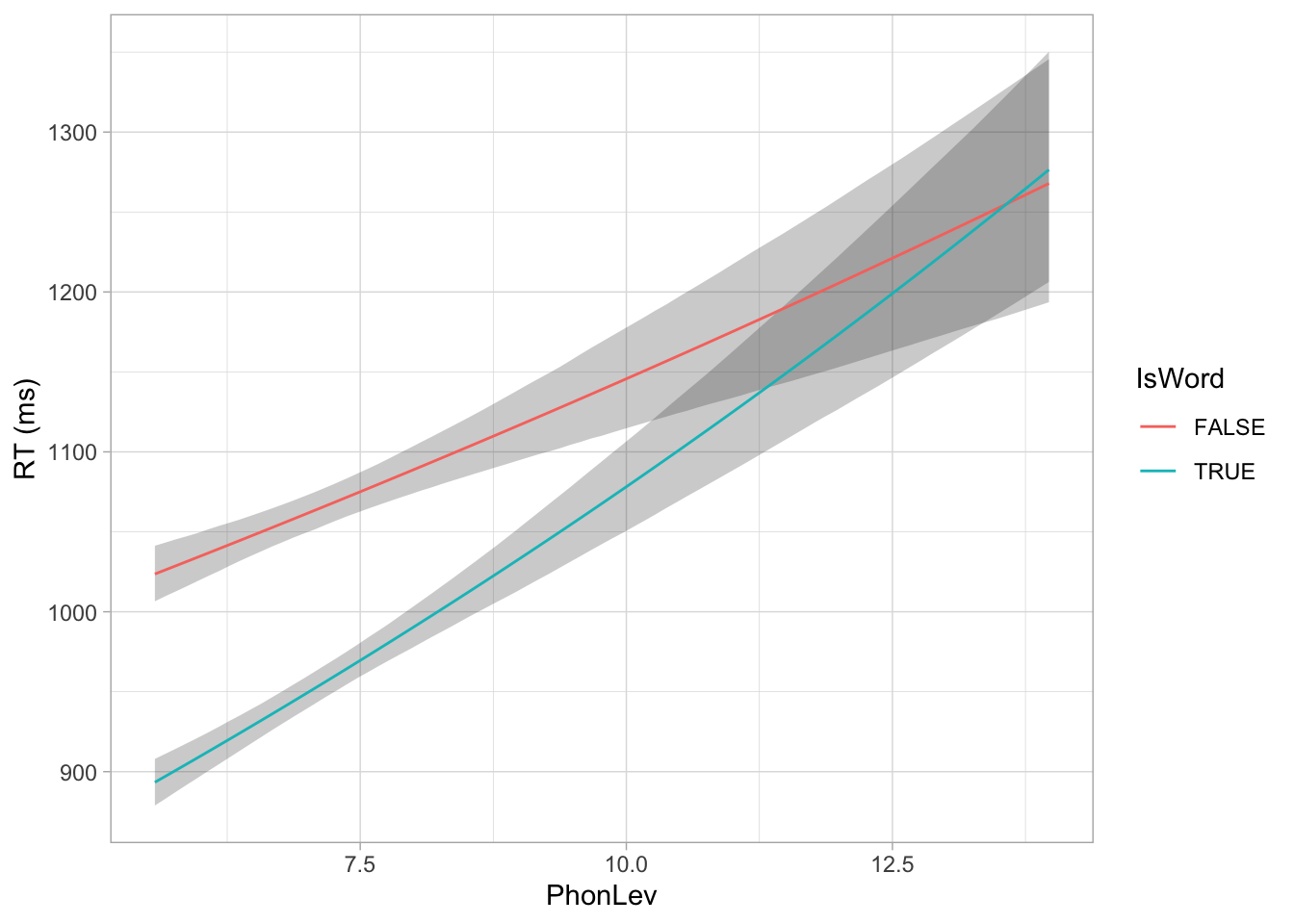
For quick plotting, you can also use conditional_effects() as we have seen above.
conditional_effects(mald_bm, "PhonLev:IsWord")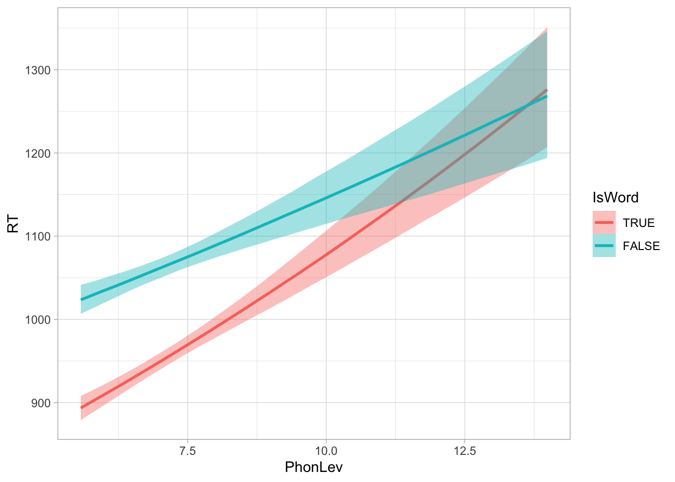
4 Summary
References
Bürkner, Paul-Christian. 2017. Brms: An r package for bayesian multilevel models using stan. Journal of Statistical Software 80(1). 128. https://doi.org/10.18637/jss.v080.i01.
McLaughlin, Drew J., Maggie E. Zink, Lauren Gaunt, Brent Spehar, Kristin J. Van Engen, Mitchell S. Sommers & Jonathan E. Peelle. 2022. Pupillometry reveals cognitive demands of lexical competition during spoken word recognition in young and older adults. Psychonomic Bulletin & Review 29(1). 268–280. https://doi.org/10.3758/s13423-021-01991-0. https://link.springer.com/10.3758/s13423-021-01991-0.
Tucker, Benjamin V, Daniel Brenner, Kyle Danielson D, Matthew C Kelley, Filip Nenadić & Michelle Sims. 2019. The massive auditory lexical decision (MALD) database. Behavior Research Methods 51(3). 11871204. https://doi.org/10.3758/s13428-018-1056-1.
Citation
BibTeX citation:
@online{coretta2025,
  author = {Coretta, Stefano},
  title = {Obtaining Expected Values from the Posterior Predictive
    Distribution in Brms Models},
  date = {2025-11-08},
  url = {https://stefanocoretta.github.io/posts/2025-11-08-expected-predictions/},
  langid = {en}
}
For attribution, please cite this work as:
Coretta, Stefano. 2025. Obtaining expected values from the posterior
predictive distribution in brms models. https://stefanocoretta.github.io/posts/2025-11-08-expected-predictions/.