n_o <- 150
se_o <- 10
se_e <- 5

n_e <- ( ( sqrt(n_o) * se_o ) / se_e )^2
n_e
[1] 600This post shows how to do a quick and dirty Bayesian power analysis.
“Power” analysis might not be a very appropriate term when Bayesian statistics is concerned. A good alternative could be “precision” analysis, since the method presented in this post is about estimate precision.
More specifically, the aim of this type of analysis is to find the approximate minimum sample size required to reach a given level of precision. By precision, I mean the width of the posterior probability of the effect of interest and, by corollary, the widths of its Credible Intervals (CrI). The smaller the width of posterior/CrI, the greater the precision of the estimate.
To calculate the minimum sample size for a particular precision value, we can take advantage of the formula of the standard error of the mean:
\[ se = \frac{\sigma}{\sqrt{n}} \]
where \(se\) is the standard error of the mean, \(\sigma\) is the sample standard deviation and \(n\) is the sample size.
Note that in Bayesian statistics, the \(se\) is the standard deviation of the posterior probability of the effect of interest.
In the scenario of a power analysis, we want to know which \(n_e\) we need to get a specific \(se_e\). We can calculate the expected sample size \(n_e\) to get a specific \(se_e\) by plugging in the observed \(se_o\), the known sample size \(n_o\) and the chosen \(se_e\), in the following formula (which is derived from the standard error formula above).
\[ n_e = \left( \frac{\sqrt{n_o} \times se_o}{se_e}\right)^2 \]
Let’s see how to calculate \(n_e\).
Imagine you have fitted a Bayesian linear model to f0 values with formality as a predictor (formal vs informal speech). Let’s say the posterior probability of the effect of formality has a 95% CrI = [-10, +30] Hz, meaning that the standard deviation is 10 Hz. In total, there were 150 data points.
So, the observed standard error (i.e. the standard deviation of the posterior) is \(se_o = 10\), the sample size is \(n_o = 150\).
Then we need to choose the standard error \(se_e\) we would want to be able to get if we ran a second iteration of the study. Let’s say we want an \(se_e\) of 5 Hz. Now, which is the \(n_e\) we need to get \(se_e = 5\)?
Easy! We just plug in the numbers to get \(n_e\).
n_o <- 150
se_o <- 10
se_e <- 5
n_e <- ( ( sqrt(n_o) * se_o ) / se_e )^2
n_e[1] 600The sample size required to go from an \(se_o\) of 10 Hz to an \(se_e\) of 4 Hz is 600. 😱
So to get an \(se\) that is half of the observed one we would need 4 times the number of data points.
Let’s spice our coding up a bit and write a few functions we can use to calculate samples sizes for different &se_e$s.
Also, so far we’ve been talking about \(se_e\) or, in other words, the standard deviation of the of the posterior probability of the effect of interest. If you remember your probability 101, you should know that the width of the 95% CrI of a posterior probability is 4 times the standard deviation.
So let’s write a function to calculate \(n_e\) based on the width of the 95% CrI, rather than on the \(se_e\).
estimate_n <- function(obs_se, obs_n, width, divide = 1) {
  sigma <- sqrt(obs_n) * obs_se
  se <- width / 4
  new_n <- (sigma / se)^2
  return(new_n / divide)
}
Let’s take it for a spin, using the numbers from the example above. The \(se_o\) we observed was 10 Hz, that’s corresponds to a width of \(10 * 4 = 40\) Hz. (Note that the first argument is the \(se_o\), not the width, but you can change that for consistency if you wish). The sample size \(n_o\) was 150. The \(se_e\) we want was 5 Hz, so the width is \(5 * 4 = 20\) Hz.
Let’s plug in these numbers.
estimate_n(obs_se = 10, obs_n = 150, width = 20)[1] 600As we have already seen above, to get a 95% CrI width of 20 Hz, we would need at least 600 observations.
Now let’s define a few functions that calculate the required sample size at different widths and create a plot.
get_obs_range <- function(obs_se, obs_n, min_width = 1, max_width, by = 1, divide = 1) {
  obs_range <- NULL
  for (i in seq(min_width, max_width, by = by)) {
    obs_range <- c(obs_range, estimate_n(obs_se, obs_n, i, divide))
  }
  return(obs_range)
}

plot_obs_range <- function(obs_se, obs_n, min_width = 1, max_width, by = 1, divide = 1) {
  obs_range <- get_obs_range(obs_se, obs_n, min_width, max_width, by, divide)

  ggplot2::ggplot() +
    aes(x = seq(min_width, max_width, by = by), y = obs_range) +
    geom_point() +
    geom_path() +
    labs(
      caption = paste0("SE = ", obs_se, ", ", obs_n, " obs"),
      x = "CI width",
      y = paste0("Estimated N ", "(N/", divide, ")")
    )
}
Let’s now plot the required sample sizes to reach a 95% CrI width in the range from 10 to 50, by 5.
plot_obs_range(10, 150, min_width = 10, max_width = 50, by = 5) +
  scale_y_continuous(breaks = seq(0, 3000, 250))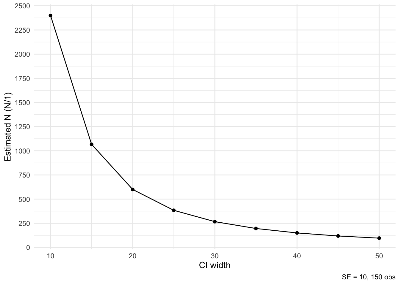
@online{coretta2022,
  author = {Coretta, Stefano},
  title = {Bayesian {CrI-width} Power Analysis},
  date = {2022-04-05},
  url = {https://stefanocoretta.github.io/posts/2022-04-05-bayesian-ci-width-power-analysis/},
  langid = {en}
}