Vowel formants trajectories and tidy data

With the advent of more powerful statistical methods for assessing time series data, it is now becoming more common to compare whole vowel formant trajectories rather then just using average values.

In this post I will show how to tidy a formant measurements dataset and plot formants using the tidyverse (Wickham 2017).

From wide to long

To illustrate the process, I will use formant data that was kindly provided by Stephen Nichols.

Let’s first read in the data.

trajectories <- read_csv("./data/nichols-2018/tulemupepelako.csv")

trajectories

# A tibble: 7 × 61
   Time Vowel Word      Duration F1_05 F1_10 F1_15 F1_20 F1_25 F1_30 F1_35 F1_40
  <dbl> <chr> <chr>        <dbl> <dbl> <dbl> <dbl> <dbl> <dbl> <dbl> <dbl> <dbl>
1  194. u     tulemupe…     43.3  406.  439.  453.  456.  430.  357.  314.  288.
2  194. e     tulemupe…    103.   503.  517.  537.  564.  556.  362.  315.  295.
3  194. u     tulemupe…     14.1  290.  288.  286.  283.  281.  281.  282.  295.
4  194. e     tulemupe…     75.7  440.  441.  439.  429.  386.  269.  250.  318.
5  194. e     tulemupe…     68.2  437.  445.  479.  562.  622.  605.  523.  618.
6  195. a     tulemupe…     89.8  800.  736.  662.  543.  447.  564.  768.  358.
7  195. o     tulemupe…     98.5  482.  463.  471.  326.  316.  573. 1511. 1389.
# ℹ 49 more variables: F1_45 <dbl>, F1_50 <dbl>, F1_55 <dbl>, F1_60 <dbl>,
#   F1_65 <dbl>, F1_70 <dbl>, F1_75 <dbl>, F1_80 <dbl>, F1_85 <dbl>,
#   F1_90 <dbl>, F1_95 <dbl>, F2_05 <dbl>, F2_10 <dbl>, F2_15 <dbl>,
#   F2_20 <dbl>, F2_25 <dbl>, F2_30 <dbl>, F2_35 <dbl>, F2_40 <dbl>,
#   F2_45 <dbl>, F2_50 <dbl>, F2_55 <dbl>, F2_60 <dbl>, F2_65 <dbl>,
#   F2_70 <dbl>, F2_75 <dbl>, F2_80 <dbl>, F2_85 <dbl>, F2_90 <dbl>,
#   F2_95 <dbl>, F3_05 <dbl>, F3_10 <dbl>, F3_15 <dbl>, F3_20 <dbl>, …

The dataset contains formant values of F1-F3 at 5% intervals for the vowels in the word tulemupepelako ‘we are praying for her’ (Bemba, [bemb1257]).

In the first step, we will create two columns, one with the formant/interval label and one with the formant value, using pivot_longer().

trajectories_long <- pivot_longer(
  trajectories,
  F1_05:F3_95,
  names_to = "formant_int",
  values_to = "value")

trajectories_long

# A tibble: 399 × 6
    Time Vowel Word           Duration formant_int value
   <dbl> <chr> <chr>             <dbl> <chr>       <dbl>
 1  194. u     tulemupepelako     43.3 F1_05        406.
 2  194. u     tulemupepelako     43.3 F1_10        439.
 3  194. u     tulemupepelako     43.3 F1_15        453.
 4  194. u     tulemupepelako     43.3 F1_20        456.
 5  194. u     tulemupepelako     43.3 F1_25        430.
 6  194. u     tulemupepelako     43.3 F1_30        357.
 7  194. u     tulemupepelako     43.3 F1_35        314.
 8  194. u     tulemupepelako     43.3 F1_40        288.
 9  194. u     tulemupepelako     43.3 F1_45        286.
10  194. u     tulemupepelako     43.3 F1_50        327.
# ℹ 389 more rows

The next step is to separate the formant_int column into two columns: one for formant, and one for interval. The argument convert = TRUE ensures that the interval column is converted into a numeric column.

trajectories_sep <- separate(
  trajectories_long,
  formant_int,
  c("formant", "interval"),
  convert = TRUE
)

trajectories_sep

# A tibble: 399 × 7
    Time Vowel Word           Duration formant interval value
   <dbl> <chr> <chr>             <dbl> <chr>      <int> <dbl>
 1  194. u     tulemupepelako     43.3 F1             5  406.
 2  194. u     tulemupepelako     43.3 F1            10  439.
 3  194. u     tulemupepelako     43.3 F1            15  453.
 4  194. u     tulemupepelako     43.3 F1            20  456.
 5  194. u     tulemupepelako     43.3 F1            25  430.
 6  194. u     tulemupepelako     43.3 F1            30  357.
 7  194. u     tulemupepelako     43.3 F1            35  314.
 8  194. u     tulemupepelako     43.3 F1            40  288.
 9  194. u     tulemupepelako     43.3 F1            45  286.
10  194. u     tulemupepelako     43.3 F1            50  327.
# ℹ 389 more rows

Now we can put back the formant labels into one column each. We can achieve this with pivot_wider(), the counterpart of pivo_longer().

trajectories_wide <- pivot_wider(
  trajectories_sep,
  names_from = formant,
  values_from = value
)

trajectories_wide

# A tibble: 133 × 8
    Time Vowel Word           Duration interval    F1    F2    F3
   <dbl> <chr> <chr>             <dbl>    <int> <dbl> <dbl> <dbl>
 1  194. u     tulemupepelako     43.3        5  406. 1205. 2626.
 2  194. u     tulemupepelako     43.3       10  439. 1226. 2556.
 3  194. u     tulemupepelako     43.3       15  453. 1246. 2507.
 4  194. u     tulemupepelako     43.3       20  456. 1291. 2451.
 5  194. u     tulemupepelako     43.3       25  430. 1418. 2331.
 6  194. u     tulemupepelako     43.3       30  357. 1555. 2268.
 7  194. u     tulemupepelako     43.3       35  314. 1603. 2335.
 8  194. u     tulemupepelako     43.3       40  288. 1709. 2437.
 9  194. u     tulemupepelako     43.3       45  286. 1712. 2461.
10  194. u     tulemupepelako     43.3       50  327. 1747. 2470.
# ℹ 123 more rows

We now have a dataset with separate columns for each formant and individual rows for each vowel interval.

The pipe

All the individual steps above can be chained by using the pipe %>%. What the pipe does is simply “transferring” the output of the function before it as the input of the function after it.

trajectories <- trajectories %>%
  pivot_longer(F1_05:F3_95, names_to = "formant_int", values_to = "value") %>%
  separate(formant_int, c("formant", "interval"), convert = TRUE) %>%
  pivot_wider(names_from = formant, values_from = value)

Plot

We can finally plot the formant trajectories.

trajectories %>%
  ggplot(aes(x = interval)) +
  geom_smooth(aes(y = F1), method = "gam", se = FALSE, colour = "#A7473A") +
  geom_smooth(aes(y = F2), method = "gam", se = FALSE, colour = "#4B5F6C") +
  geom_smooth(aes(y = F3), method = "gam", se = FALSE, colour = "#B09B37") +
  facet_wrap(~ Vowel) +
  ylab("Hertz")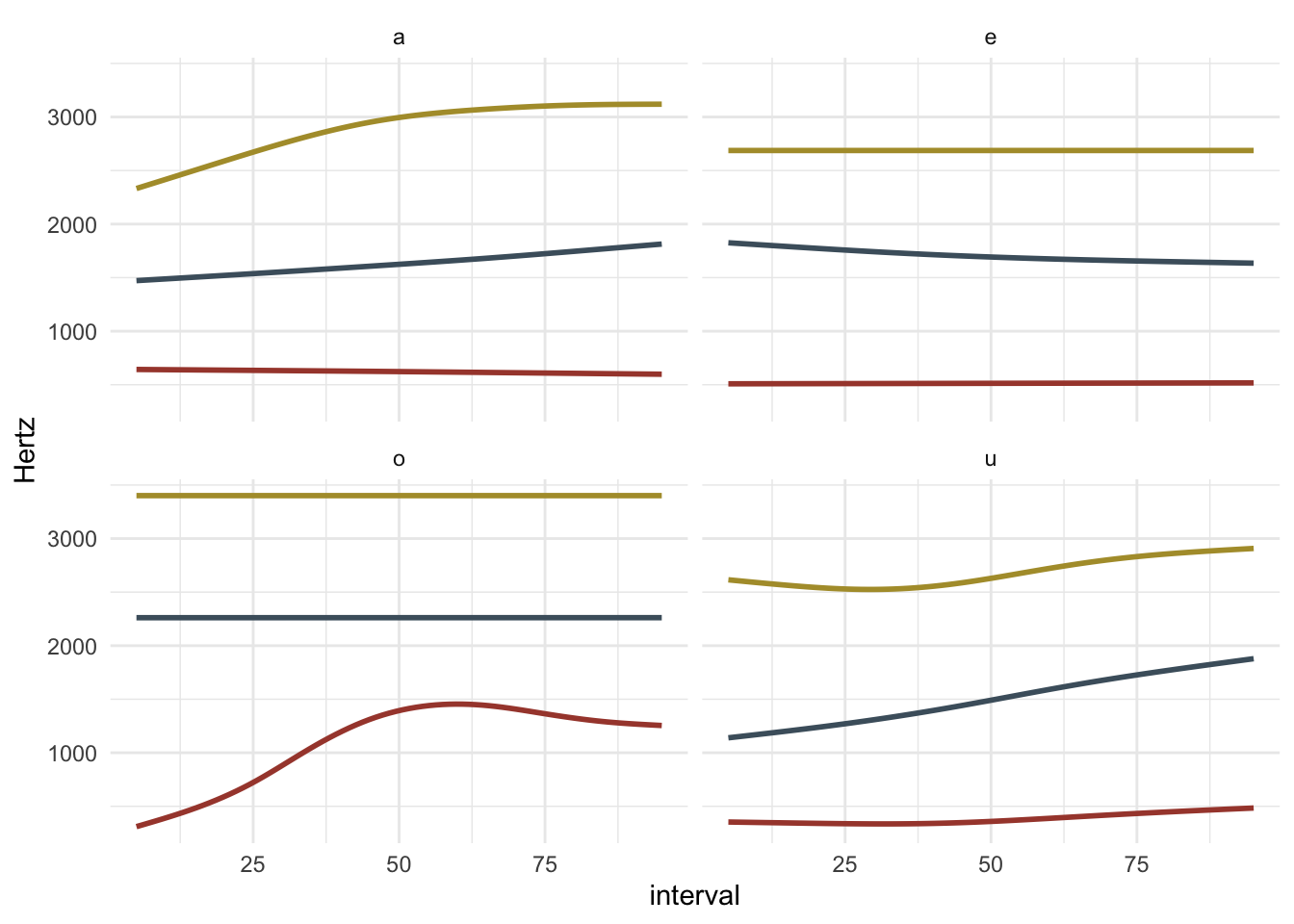

References

Wickham, Hadley. 2017. tidyverse: Easily install and load the tidyverse. R package version 1.2.1.