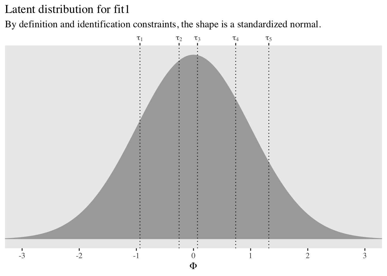
Ordinal regression models for Likert/rating scales data

Dr Stefano Coretta

University of Edinburgh

2025-01-23

Ordinal data

acceptability <- read_csv("https://osf.io/download/xmkvg/")
acceptability |> select(Participant, Condition, Response)
# A tibble: 1,176 × 3
   Participant Condition    Response
   <chr>       <chr>           <dbl>
 1 g1          canonical           7
 2 g1          noncanonical        7
 3 g1          canonical           7
 4 g1          noncanonical        7
 5 g1          canonical           7
 6 g1          noncanonical        6
 7 g1          canonical           7
 8 g1          noncanonical        7
 9 g1          canonical           6
10 g1          noncanonical        7
# ℹ 1,166 more rows

Process data for plotting

acceptability_lik <- acceptability |>
  # we count the numbers for each Condition and Response combo
  count(Condition, Response) |>
  # then we pivot so that the data is wider, with columns for condition and 
  # each of the 7 values for the Response
  pivot_wider(names_from = "Response", values_from = n)
acceptability_lik
# A tibble: 2 × 8
  Condition      `1`   `2`   `3`   `4`   `5`   `6`   `7`
  <chr>        <int> <int> <int> <int> <int> <int> <int>
1 canonical        2     6     4    25    42   164   345
2 noncanonical     8    25    22    46    88   157   242

Diverging stacked bar chart

HH::likert(
  Condition ~ .,
  acceptability_lik,
  as.percent = TRUE,
  main = "Acceptability ratings by sentence condition"
)

Ordinal variables are categorical

Ordinal variables are categorical: Gaussian regression fails

Cumulative ordinal regression models

Modelling acceptability with a cumulative ordinal model

acc_bm_1 <- brm(
  Response ~ Condition + (Condition | Participant) + (1 | Item),
  data = acceptability,
  family = cumulative("probit"),
  cores = 4,
  seed = 7823,
  file = "data/cache/acc_bm_1"
)

Modelling acceptability: summary

summary(acc_bm_1)
 Family: cumulative 
  Links: mu = probit; disc = identity 
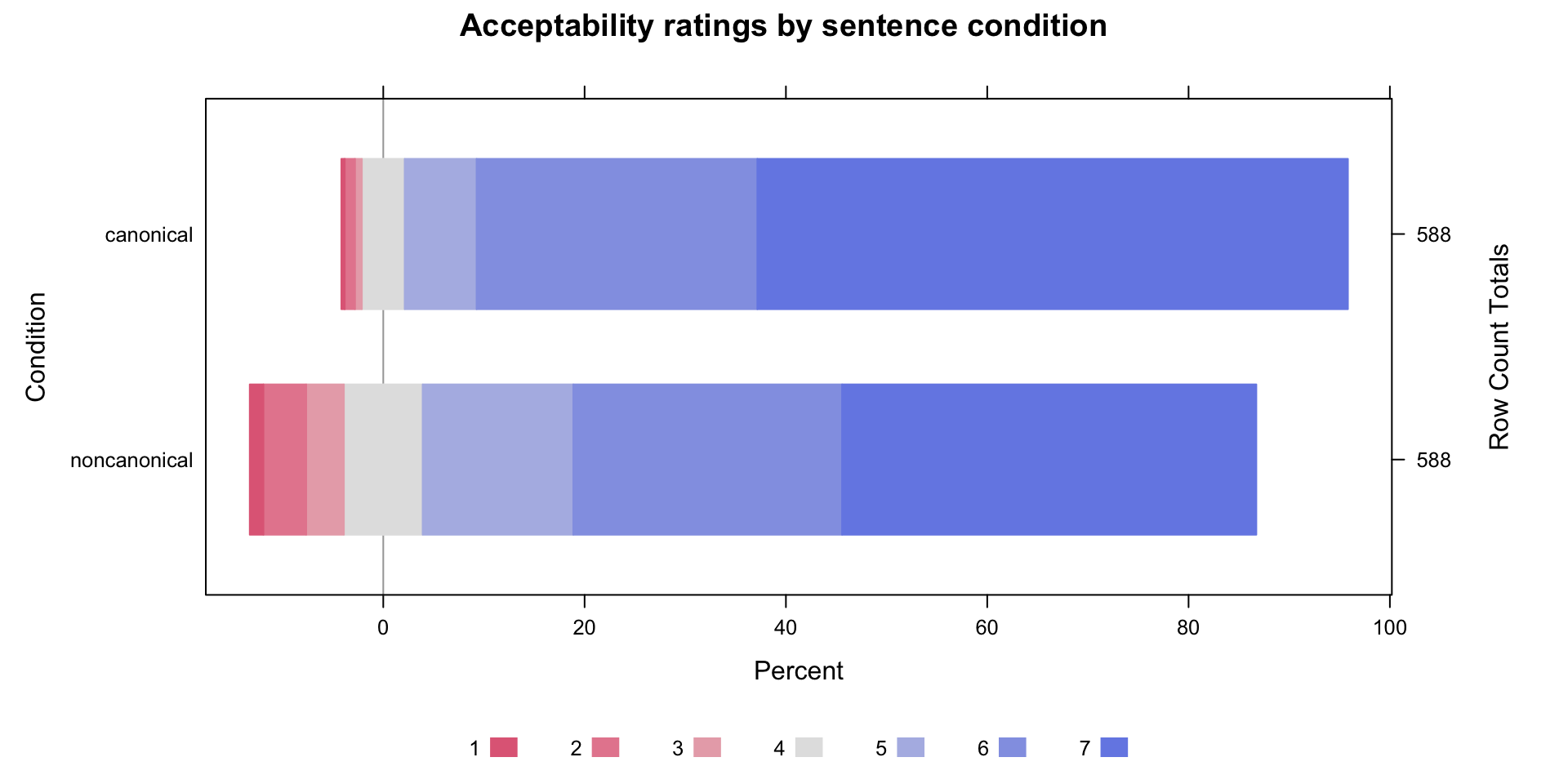
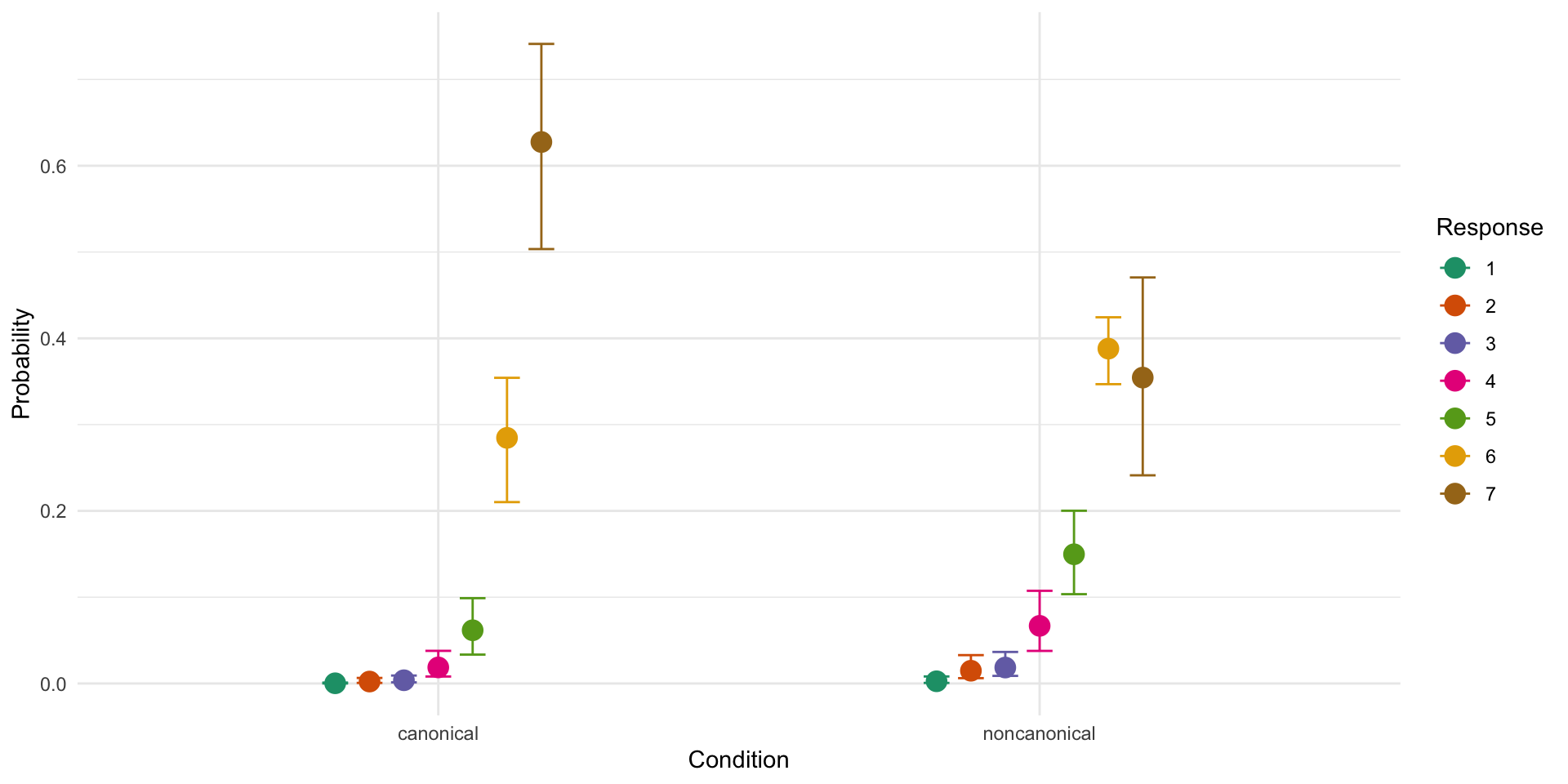
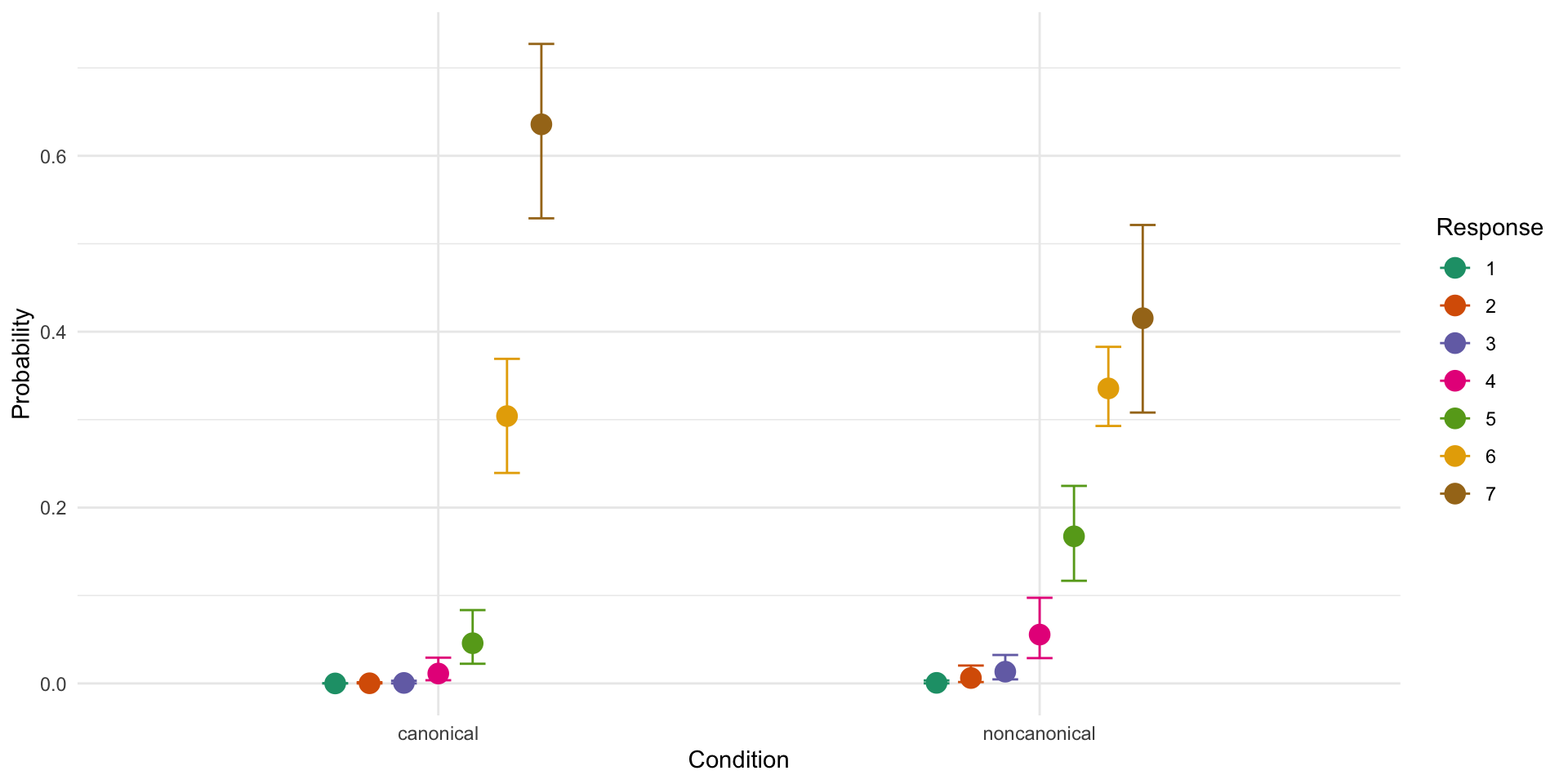
Formula: Response ~ Condition + (Condition | Participant) + (1 | Item) 
   Data: acceptability (Number of observations: 1176) 
  Draws: 4 chains, each with iter = 2000; warmup = 1000; thin = 1;
         total post-warmup draws = 4000

Multilevel Hyperparameters:
~Item (Number of levels: 28) 
              Estimate Est.Error l-95% CI u-95% CI Rhat Bulk_ESS Tail_ESS
sd(Intercept)     0.36      0.07     0.25     0.50 1.00     1430     1825

~Participant (Number of levels: 42) 
                                     Estimate Est.Error l-95% CI u-95% CI Rhat
sd(Intercept)                            0.89      0.13     0.68     1.18 1.00
sd(Conditionnoncanonical)                0.33      0.13     0.05     0.57 1.00
cor(Intercept,Conditionnoncanonical)    -0.20      0.32    -0.76     0.49 1.00
                                     Bulk_ESS Tail_ESS
sd(Intercept)                             805     1735
sd(Conditionnoncanonical)                 596      528
cor(Intercept,Conditionnoncanonical)     1823     1347

Regression Coefficients:
                      Estimate Est.Error l-95% CI u-95% CI Rhat Bulk_ESS
Intercept[1]             -3.50      0.22    -3.94    -3.09 1.00      903
Intercept[2]             -2.81      0.19    -3.18    -2.45 1.00      825
Intercept[3]             -2.49      0.18    -2.86    -2.14 1.00      803
Intercept[4]             -1.96      0.18    -2.32    -1.62 1.00      752
Intercept[5]             -1.36      0.17    -1.70    -1.04 1.01      722
Intercept[6]             -0.33      0.17    -0.65    -0.01 1.01      699
Conditionnoncanonical    -0.70      0.09    -0.89    -0.53 1.00     2456
                      Tail_ESS
Intercept[1]              1876
Intercept[2]              1444
Intercept[3]              1444
Intercept[4]              1475
Intercept[5]              1350
Intercept[6]              1575
Conditionnoncanonical     2602

Further Distributional Parameters:
     Estimate Est.Error l-95% CI u-95% CI Rhat Bulk_ESS Tail_ESS
disc     1.00      0.00     1.00     1.00   NA       NA       NA

Draws were sampled using sampling(NUTS). For each parameter, Bulk_ESS
and Tail_ESS are effective sample size measures, and Rhat is the potential
scale reduction factor on split chains (at convergence, Rhat = 1).

Modelling acceptability: regression coefficients

fixef(acc_bm_1)
                        Estimate  Est.Error       Q2.5       Q97.5
Intercept[1]          -3.5026028 0.21929110 -3.9384487 -3.08514908
Intercept[2]          -2.8072746 0.18963455 -3.1834800 -2.44661624
Intercept[3]          -2.4948545 0.18212668 -2.8573013 -2.14070922
Intercept[4]          -1.9616831 0.17659995 -2.3177691 -1.62034369
Intercept[5]          -1.3619645 0.17027364 -1.7022029 -1.04122602
Intercept[6]          -0.3252862 0.16589856 -0.6470002 -0.00858996
Conditionnoncanonical -0.7023993 0.09175824 -0.8880742 -0.52622744
  • Each “intercept” is the estimated threshold between the Nth category and the following category, on the latent standard Gaussian distribution.

    \[ Pr(Y = k) = \Phi(\tau_k) - \Phi(\tau_{k-1}) \]

  • Conditionnoncaconical indicates how the acceptability scores differ in the non-canonical condition relative to the canonical one on the latent Gaussian distribution.

  • Negative values of Conditionnoncaconical indicate lower acceptability.

Modelling acceptability: predicted acceptability

conditional_effects(acc_bm_1, categorical = TRUE)

Category-specific effects

  • Cumulative models assume a single latent variable.

  • Moreover, there is only one parameter for Condition which shifts the entire latent variable but does not allow for rating-category-specific differences.

  • We can use adjacent category models with category-specific effects.

Category-specific effects: fit adjacent category model

acc_bm_2 <- brm(
  Response ~ cs(Condition) + (Condition | Participant) + (1 | Item),
  data = acceptability,
  family = acat("probit"),
  cores = 4,
  seed = 7823,
  file = "data/cache/acc_bm_2"
)

Category-specific effects: model summary

acc_bm_2_fixef <- fixef(acc_bm_2)
round(acc_bm_2_fixef, 2)
                         Estimate Est.Error  Q2.5 Q97.5
Intercept[1]                -1.43      0.49 -2.45 -0.51
Intercept[2]                -0.62      0.38 -1.34  0.12
Intercept[3]                -1.65      0.29 -2.22 -1.09
Intercept[4]                -0.85      0.19 -1.22 -0.48
Intercept[5]                -1.12      0.15 -1.42 -0.84
Intercept[6]                -0.46      0.11 -0.68 -0.23
Conditionnoncanonical[1]    -0.14      0.54 -1.24  0.87
Conditionnoncanonical[2]    -0.14      0.41 -0.93  0.67
Conditionnoncanonical[3]    -0.78      0.32 -1.41 -0.16
Conditionnoncanonical[4]    -0.17      0.21 -0.58  0.24
Conditionnoncanonical[5]    -0.69      0.15 -0.98 -0.41
Conditionnoncanonical[6]    -0.33      0.10 -0.53 -0.13
  • Each “intercept” is the threshold between the Nth level and the following level.

    \[ P(Y = k \mid \eta) = \frac{\exp\left(\sum_{j=1}^{k-1} (\eta - \tau_j)\right)}{\sum_{r=1}^{K+1} \exp\left(\sum_{j=1}^{r-1} (\eta - \tau_j)\right)} \]

  • Now, Condition has one coefficient per rating-category.

  • For example, Conditionnoncanonical[6] with a 95% CrI [-0.53, -0.13] indicates that in the non-canonical condition, participants favour “7” over “6” less than in the canonical condition.

Category-specific effects: predicted probabilities

conditional_effects(acc_bm_2, categorical = TRUE)

Language proficiency

proficiency <- read_csv("https://osf.io/download/4j3r2/") |> 
  mutate(
    Response = ordered(Response, levels = c("functional", "good", "very good", "nativelike"))
  )

proficiency
# A tibble: 55 × 3
   Participant Response     AoA
   <chr>       <ord>      <dbl>
 1 BLP523      very good     19
 2 CCZ257      very good     17
 3 DSY144      nativelike     7
 4 FLP885      good          18
 5 GFJ452      very good     19
 6 GLF239      nativelike    10
 7 GNB157      nativelike     7
 8 GPR735      good          10
 9 GWL482      very good     17
10 GZV988      nativelike    12
# ℹ 45 more rows

Language proficiency: plot

proficiency |>
  ggplot(aes(AoA)) +
  geom_histogram(binwidth = 2)

Language proficiency: fit model

pro_bm_1 <- brm(
  Response ~ AoA,
  data = proficiency,
  family = cumulative("probit"),
  cores = 4,
  seed = 3546,
  file = "data/cache/pro_bm_1"
)

Language proficiency: model summary

summary(pro_bm_1)
 Family: cumulative 
  Links: mu = probit; disc = identity 
Formula: Response ~ AoA 
   Data: proficiency (Number of observations: 55) 
  Draws: 4 chains, each with iter = 2000; warmup = 1000; thin = 1;
         total post-warmup draws = 4000

Regression Coefficients:
             Estimate Est.Error l-95% CI u-95% CI Rhat Bulk_ESS Tail_ESS
Intercept[1]    -4.40      0.65    -5.73    -3.20 1.00     1701     1460
Intercept[2]    -2.62      0.51    -3.63    -1.64 1.00     2317     2172
Intercept[3]    -1.41      0.43    -2.27    -0.56 1.00     3079     2983
AoA             -0.15      0.03    -0.22    -0.09 1.00     2486     2289

Further Distributional Parameters:
     Estimate Est.Error l-95% CI u-95% CI Rhat Bulk_ESS Tail_ESS
disc     1.00      0.00     1.00     1.00   NA       NA       NA

Draws were sampled using sampling(NUTS). For each parameter, Bulk_ESS
and Tail_ESS are effective sample size measures, and Rhat is the potential
scale reduction factor on split chains (at convergence, Rhat = 1).

Language proficiency: expected predictions

conditional_effects(pro_bm_1, categorical = TRUE)

A slightly more complex example: Emilian proficiency

emilian <- readRDS("data/emilianto.rds") |> 
  filter(language == "Emilian") |> 
  mutate(
    age_c = age - mean(age),
    speak_2 = ordered(speak_2)
  )
emilian |> dplyr::select(age, age_c, education, gender, speak_2)
# A tibble: 434 × 5
     age  age_c education      gender speak_2   
   <dbl>  <dbl> <fct>          <chr>  <ord>     
 1    57  23.5  Primary/Middle M      very well 
 2    20 -13.5  Secondary      F      so and so 
 3    50  16.5  Secondary      M      very well 
 4    25  -8.46 Bachelor       F      not at all
 5    65  31.5  Primary/Middle M      very well 
 6    56  22.5  Secondary      F      very well 
 7    62  28.5  Secondary      M      very well 
 8    65  31.5  Masters+       M      very well 
 9    63  29.5  Primary/Middle F      very well 
10    61  27.5  Primary/Middle M      well      
# ℹ 424 more rows

Emilian speaking competence: prepare data

emilian_lik_gen <- emilian |>
  count(gender, speak_2) |>
  pivot_wider(names_from = "speak_2", values_from = n)
emilian_lik_ed <- emilian |>
  count(education, speak_2) |>
  pivot_wider(names_from = "speak_2", values_from = n)

Emilian speaking competence by gender

Emilian speaking competence by education

Age of participants

emilian |> 
  ggplot(aes(age)) +
  geom_histogram(binwidth = 5)

Fit model

emi_bm_1 <- brm(
  speak_2 ~ cs(education) + cs(gender) + age_c,
  family = acat("probit"),
  data = emilian,
  cores = 4,
  seed = 7263,
  file = "data/cache/emi_bm_1"
)

Model summary

summary(emi_bm_1)
 Family: acat 
  Links: mu = probit; disc = identity 
Formula: speak_2 ~ cs(education) + cs(gender) + age_c 
   Data: emilian (Number of observations: 434) 
  Draws: 4 chains, each with iter = 2000; warmup = 1000; thin = 1;
         total post-warmup draws = 4000

Regression Coefficients:
                      Estimate Est.Error l-95% CI u-95% CI Rhat Bulk_ESS
Intercept[1]             -0.87      0.43    -1.76    -0.07 1.00     2081
Intercept[2]              0.34      0.31    -0.28     0.93 1.00     1739
Intercept[3]             -0.18      0.32    -0.81     0.44 1.00     1561
Intercept[4]              0.32      0.34    -0.33     1.00 1.00     1912
age_c                     0.00      0.00     0.00     0.01 1.00     5164
educationSecondary[1]    -0.02      0.44    -0.93     0.82 1.00     2251
educationSecondary[2]    -0.03      0.32    -0.64     0.60 1.00     1847
educationSecondary[3]     0.06      0.33    -0.60     0.71 1.00     1725
educationSecondary[4]    -0.13      0.35    -0.81     0.56 1.00     2058
educationBachelor[1]     -0.45      0.48    -1.42     0.49 1.00     2191
educationBachelor[2]      0.18      0.36    -0.53     0.89 1.00     1953
educationBachelor[3]     -0.17      0.39    -0.92     0.59 1.00     1719
educationBachelor[4]     -0.11      0.41    -0.90     0.68 1.00     2139
educationMastersP[1]     -0.38      0.50    -1.37     0.58 1.00     2559
educationMastersP[2]      0.29      0.37    -0.42     1.00 1.00     2148
educationMastersP[3]     -0.07      0.38    -0.82     0.67 1.00     1917
educationMastersP[4]      0.03      0.39    -0.73     0.79 1.00     2198
genderM[1]                0.50      0.26     0.01     1.03 1.00     4173
genderM[2]               -0.18      0.18    -0.54     0.17 1.00     2927
genderM[3]                0.13      0.19    -0.23     0.51 1.00     2632
genderM[4]                0.28      0.19    -0.09     0.65 1.00     3415
                      Tail_ESS
Intercept[1]              2253
Intercept[2]              1985
Intercept[3]              1964
Intercept[4]              2311
age_c                     2685
educationSecondary[1]     2447
educationSecondary[2]     2515
educationSecondary[3]     2257
educationSecondary[4]     2309
educationBachelor[1]      2482
educationBachelor[2]      2585
educationBachelor[3]      2161
educationBachelor[4]      2491
educationMastersP[1]      2803
educationMastersP[2]      2719
educationMastersP[3]      2457
educationMastersP[4]      2499
genderM[1]                2754
genderM[2]                2213
genderM[3]                2519
genderM[4]                2907

Further Distributional Parameters:
     Estimate Est.Error l-95% CI u-95% CI Rhat Bulk_ESS Tail_ESS
disc     1.00      0.00     1.00     1.00   NA       NA       NA

Draws were sampled using sampling(NUTS). For each parameter, Bulk_ESS
and Tail_ESS are effective sample size measures, and Rhat is the potential
scale reduction factor on split chains (at convergence, Rhat = 1).

Expected probabilities by gender

conditional_effects(emi_bm_1, effects = "gender", categorical = TRUE)

Expected probabilities by education

conditional_effects(emi_bm_1, effects = "education", categorical = TRUE)

Expected probabilities by age

conditional_effects(emi_bm_1, effects = "age_c", categorical = TRUE)

Resources