Introduction to Bayesian Linear Models
02 - Diagnostics
Stefano Coretta
University of Edinburgh
MCMC traces

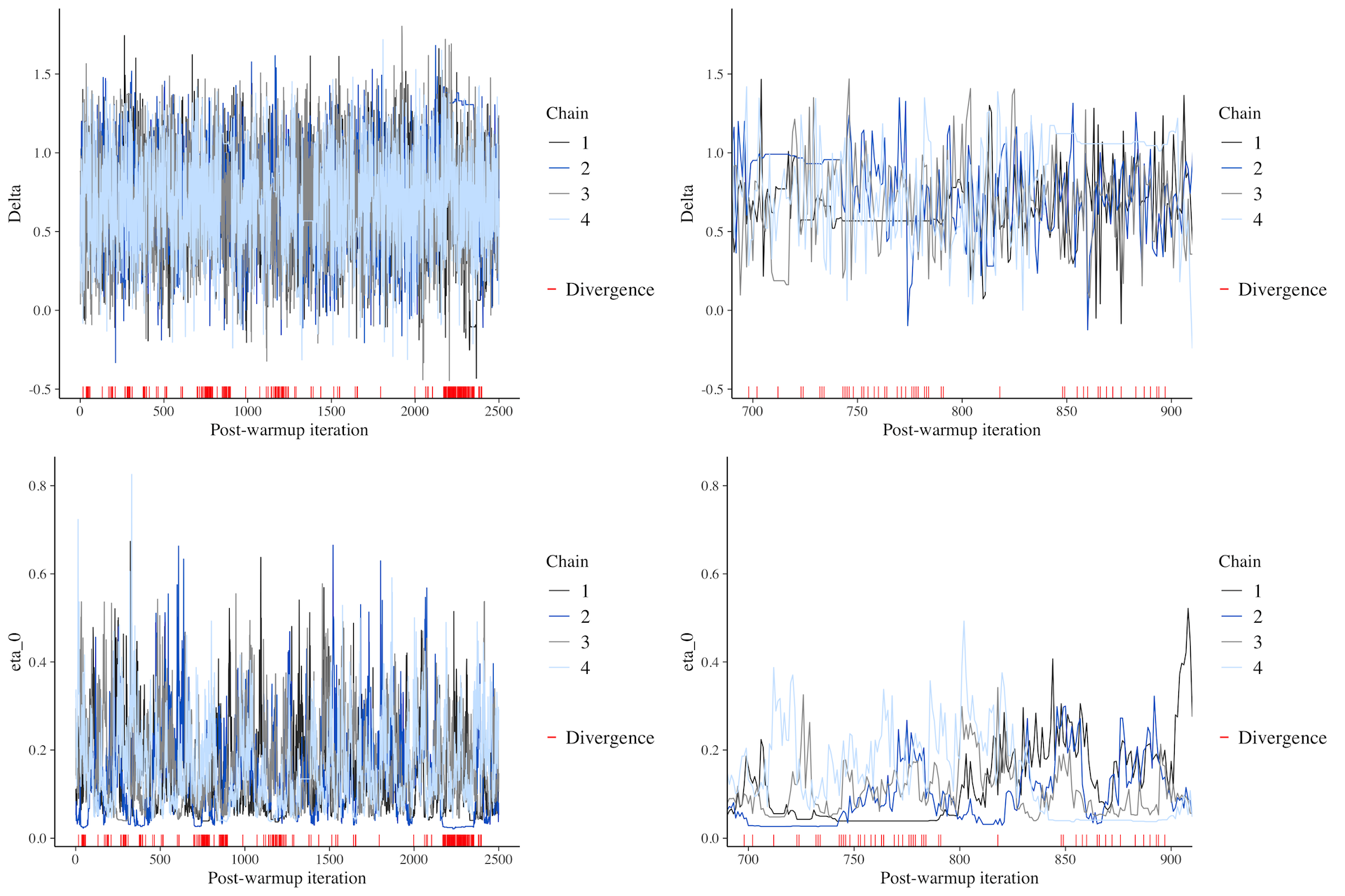
MCMC traces: bad
An example of bad MCMC chain mixing.

MCMC traces: intercept

MCMC traces: IsWord

\(\hat{R}\) and Effective Sample Size (ESS)
 Family: gaussian
  Links: mu = identity; sigma = identity
Formula: RT ~ IsWord
   Data: mald (Number of observations: 3000)
  Draws: 4 chains, each with iter = 2000; warmup = 1000; thin = 1;
         total post-warmup draws = 4000

Regression Coefficients:
            Estimate Est.Error l-95% CI u-95% CI Rhat Bulk_ESS Tail_ESS
Intercept     981.35      8.73   964.38   998.37 1.00     3970     3032
IsWordFALSE   132.87     12.63   107.91   156.87 1.00     3936     2937

Further Distributional Parameters:
      Estimate Est.Error l-95% CI u-95% CI Rhat Bulk_ESS Tail_ESS
sigma   341.21      4.48   332.33   349.82 1.00     4223     3006

Draws were sampled using sampling(NUTS). For each parameter, Bulk_ESS
and Tail_ESS are effective sample size measures, and Rhat is the potential
scale reduction factor on split chains (at convergence, Rhat = 1).
Posterior Predictive Checks

Summary
Quick and dirty diagnostics:
MCMC traces: hairy caterpillars, no divergent transitions.
\(\hat{R}\): should be 1 (> 1 means non-convergence).
Effective Sample Size (ESS): should be large enough.
Posterior Predictive Checks: predicted outcome distribution should match the empirical distribution.
brm()warns you about divergent transition, \(\hat{R} > 1\) and low ESS and how to fix them.- This usually involves increasing the number of iterations and/or other MCMC tricks.
Posterior predictive checks are based on visual inspection only.