02 - Priors

Stefano Coretta

Vowel duration

\[ \begin{align} vdur & \sim Gaussian(\mu, \sigma)\\ \end{align} \]

Pick a \(\mu\) and \(\sigma\).

Report them here: https://forms.gle/HRzH5CworngWrBv16.

Proposed distributions of vowel duration

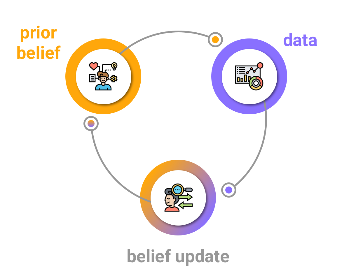
Bayesian belief update

Priors

\[ \begin{align} vdur & \sim LogNormal(\mu, \sigma)\\ \mu & \sim Gaussian(\mu_1, \sigma_1)\\ \sigma & \sim Cauchy_{+}(0, \sigma_2)\\ \end{align} \]

Get default priors

get_prior(
  v1_duration ~ 1,
  family = lognormal,
  data = token_measures
)

                  prior     class coef group resp dpar nlpar lb ub  source
 student_t(3, 4.6, 2.5) Intercept                                  default
   student_t(3, 0, 2.5)     sigma                             0    default

Prior probability distributions

The empirical rule

The empirical rule

The empirical rule

The empirical rule

The empirical rule

Priors of the model

\[ \begin{align} vdur & \sim LogNormal(\mu, \sigma)\\ \mu & \sim Gaussian(\mu_1, \sigma_1)\\ \sigma & \sim Cauchy_{+}(0, \sigma_2)\\ \end{align} \]

Let’s pick \(\mu_1\) and \(\sigma_1\).

We can use the empirical rule.

Prior for \(\mu\)

\[ \begin{align} vdur & \sim LogNormal(\mu, \sigma)\\ \mu & \sim Gaussian(\mu_1, \sigma_1)\\ \sigma & \sim Cauchy_{+}(0, \sigma_2)\\ \end{align} \]

• Let’s say that the mean vowel duration is between 50 and 150 ms at 95% confidence. In logs, that would be log(50) = 3.9 and log(150) = 5.

• Get \(\mu_1\)

  • mean(c(3.9, 5)) = 4.45

• Get \(\sigma_1\)

  • (5 - 3.9) / 4 = 0.275

Prior for \(\mu\)

\[ \begin{align} vdur & \sim LogNormal(\mu, \sigma)\\ \mu & \sim Gaussian(\mu_1 = 4.45, \sigma_1 = 0.275)\\ \sigma & \sim Cauchy_{+}(0, \sigma_2)\\ \end{align} \]

Prior for \(\mu\): plot

Prior for \(\sigma\)

library(HDInterval)

round(inverseCDF(c(0.975), ptrunc, spec = "cauchy", a = 0, scale = 0.1))

[1] 3

round(inverseCDF(c(0.975), ptrunc, spec = "cauchy", a = 0, scale = 0.2))

[1] 5

round(inverseCDF(c(0.975), ptrunc, spec = "cauchy", a = 0, scale = 0.3))

[1] 8

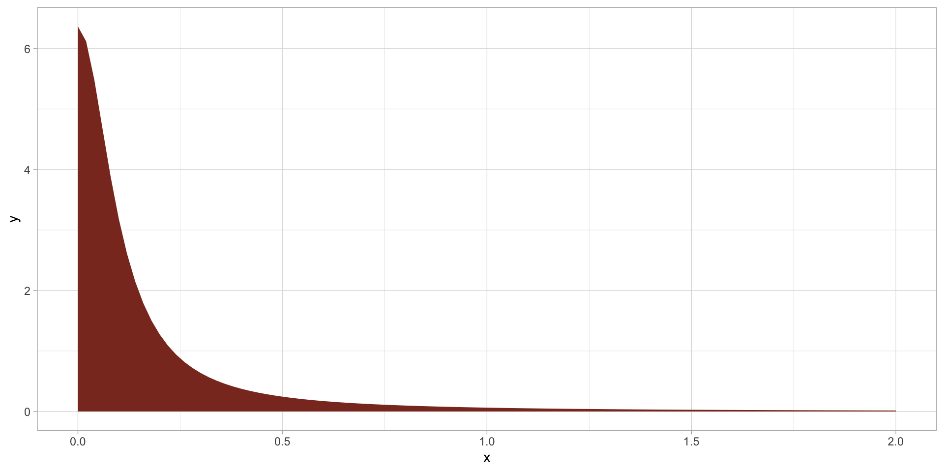
Prior for \(\sigma\): plot

ggplot(tibble(x = c(0, 2)), aes(x = x)) +
  stat_function(fun = dtrunc, geom = "area", fill = "tomato4",
                args = list(spec = "cauchy", a = 0, scale = 0.1))

Prior predictive checks: sample prior

my_seed <- 3485

m_3_priors <- c(
  prior(normal(4.45, 0.275), class = Intercept),
  prior(cauchy(0, 0.1), class = sigma)
)

m_3_priorpp <- brm(
  v1_duration ~ 1,
  family = lognormal,
  prior = m_3_priors,
  data = token_measures,
  sample_prior = "only",
  cores = 4,
  file = "data/cache/m_3_priorpp",
  seed = my_seed
)

Prior predictive checks: sample prior

summary(m_3_priorpp)

 Family: lognormal 
  Links: mu = identity; sigma = identity 
Formula: v1_duration ~ 1 
   Data: token_measures (Number of observations: 1342) 
  Draws: 4 chains, each with iter = 2000; warmup = 1000; thin = 1;
         total post-warmup draws = 4000

Regression Coefficients:
          Estimate Est.Error l-95% CI u-95% CI Rhat Bulk_ESS Tail_ESS
Intercept     4.45      0.28     3.91     5.03 1.00     2736     1915

Further Distributional Parameters:
      Estimate Est.Error l-95% CI u-95% CI Rhat Bulk_ESS Tail_ESS
sigma     0.47      3.70     0.00     2.33 1.00     2902     2096

Draws were sampled using sampling(NUTS). For each parameter, Bulk_ESS
and Tail_ESS are effective sample size measures, and Rhat is the potential
scale reduction factor on split chains (at convergence, Rhat = 1).

Prior predictive checks: plot

set.seed(my_seed)
m_3_pppreds <- posterior_predict(m_3_priorpp, newdata = tibble(y = 1), ndraws = 1e3) |>
  as.vector()

ggplot() +
  aes(x = m_3_pppreds) +
  geom_density(fill = "forestgreen") +
  geom_rug(alpha = 0.25)

Prior predictive checks: plot (zoom in)

ggplot() +
  aes(x = m_3_pppreds) +
  geom_density(fill = "forestgreen") +
  geom_rug(alpha = 0.25) +
  xlim(-100, 500)

Run the model

m_3 <- brm(
  v1_duration ~ 1,
  family = lognormal,
  prior = m_3_priors,
  data = token_measures,
  cores = 4,
  file = "data/cache/m_3",
  seed = my_seed
)

Model summary

summary(m_3, prob = 0.8)

 Family: lognormal 
  Links: mu = identity; sigma = identity 
Formula: v1_duration ~ 1 
   Data: token_measures (Number of observations: 1342) 
  Draws: 4 chains, each with iter = 2000; warmup = 1000; thin = 1;
         total post-warmup draws = 4000

Regression Coefficients:
          Estimate Est.Error l-80% CI u-80% CI Rhat Bulk_ESS Tail_ESS
Intercept     4.59      0.01     4.58     4.61 1.00     4265     3162

Further Distributional Parameters:
      Estimate Est.Error l-80% CI u-80% CI Rhat Bulk_ESS Tail_ESS
sigma     0.33      0.01     0.32     0.34 1.00     3407     2797

Draws were sampled using sampling(NUTS). For each parameter, Bulk_ESS
and Tail_ESS are effective sample size measures, and Rhat is the potential
scale reduction factor on split chains (at convergence, Rhat = 1).

Posterior predictive checks

pp_check(m_3, ndraws = 100)