Causal Inference for linguistics

Correlation is causation

Stefano Coretta

University of Edinburgh

2026-05-20

“Correlation is not causation”

Photo by Courtney Cook on Unsplash

Clothing and ice cream

🎽 shorter clothing ↔︎️ more ice cream 🍨

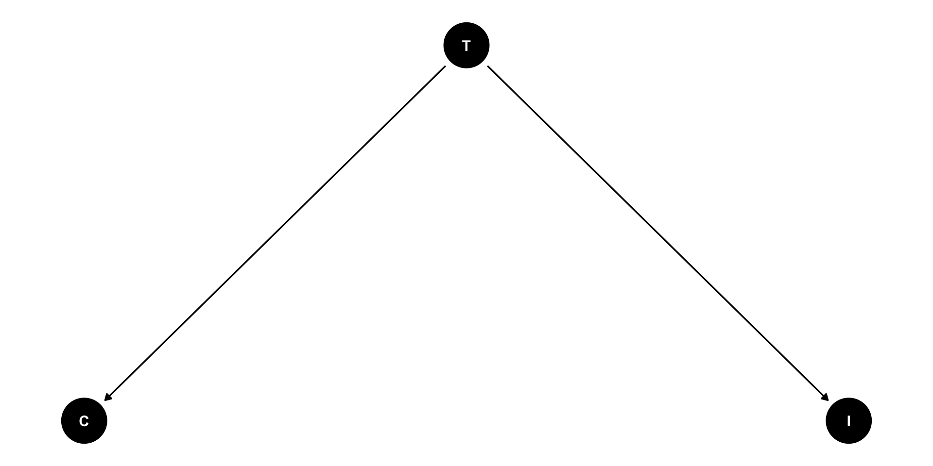
Confound: temperature

🌡️ higher temperature ➡️ shorter clothing 🎽

🌡️ higher temperature ➡️ more ice cream 🍨

Causal effects

Directed acyclic graphs (DAGs)

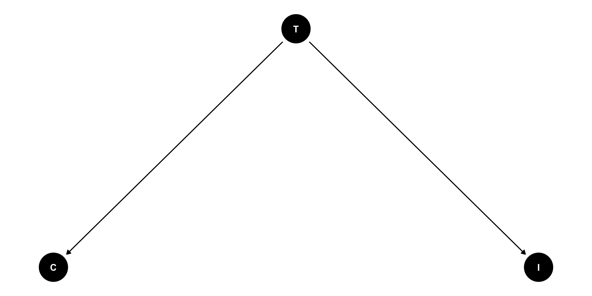
• Graphical causal theory.

• Nodes represent variables.

• Edges (arrows) represent causal effects (directed).

• Causality flows “linearly”, no circular causality (acylic).

Sentence length and subordination frequency

C = discourse complexity, L = sentence length, S = subordination frequency. Pander Maat (2017)

Four path types

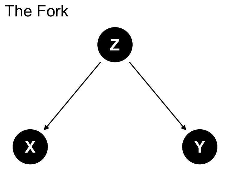
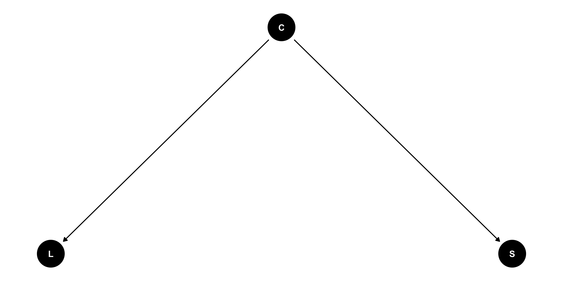
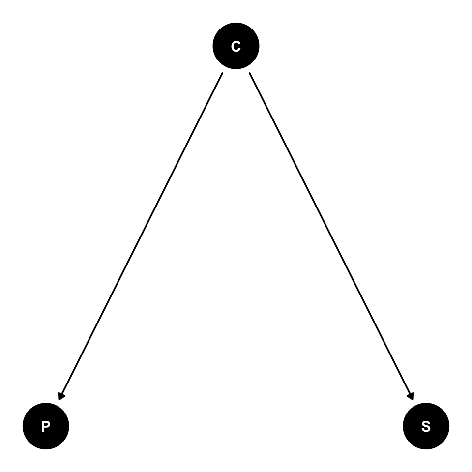
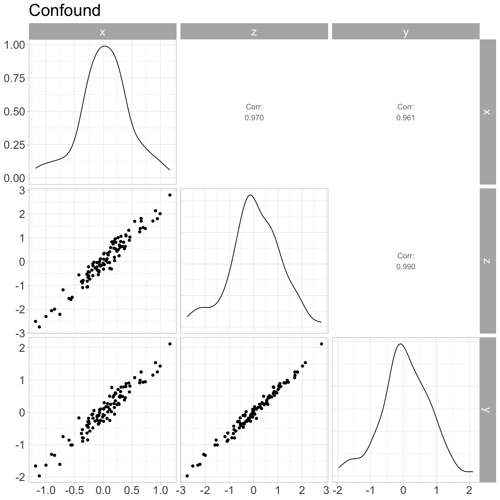
The Fork: Z is a confound

Confound: simulate

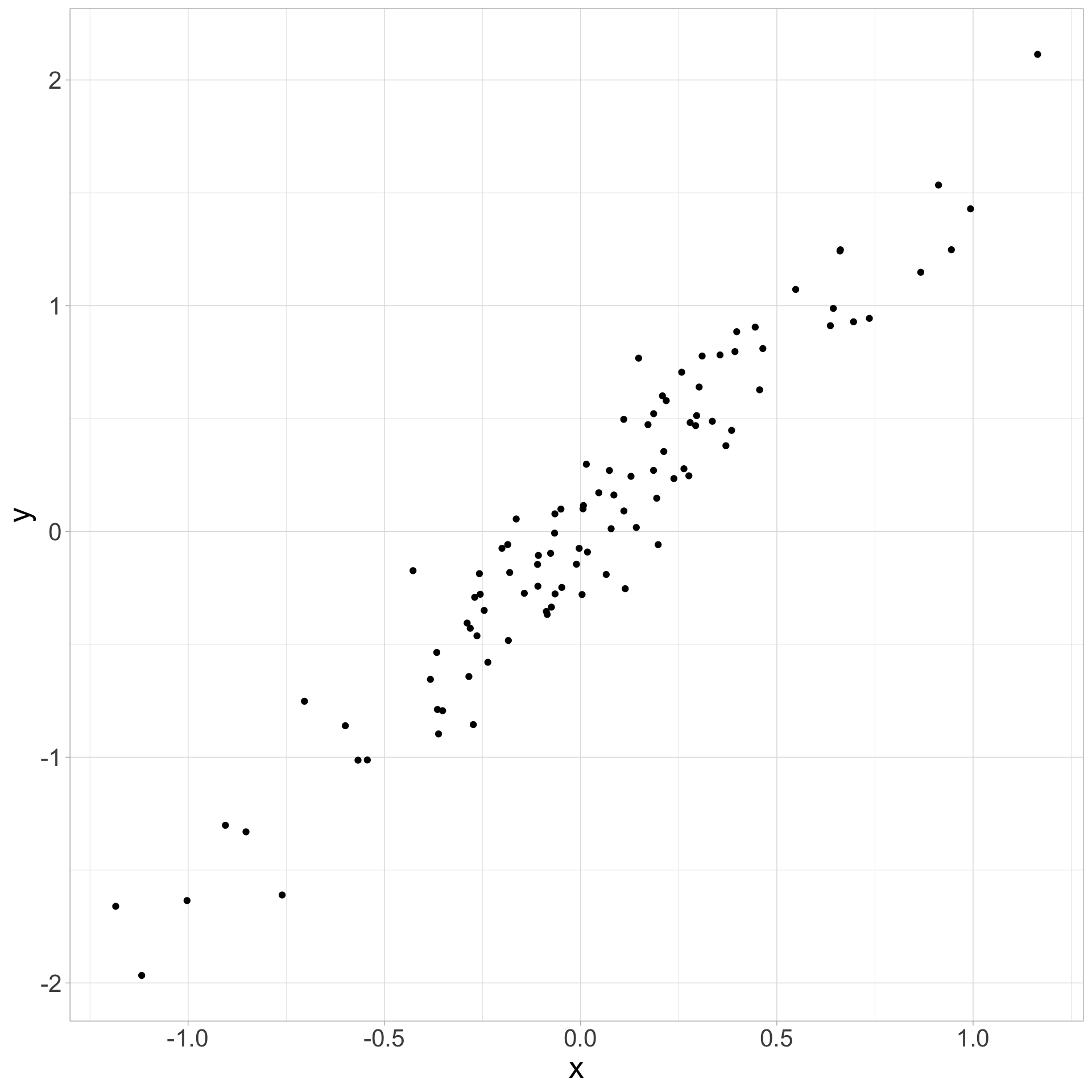
set.seed(9988)

n <- 100

z <- rnorm(n)

x <- 0.4 * z + rnorm(n, 0, 0.1)
y <- 0.7 * z + rnorm(n, 0, 0.1)

Confound: greater proficiency and code-switching

P = proficiency, S = code-switching. Schächinger Tenés et al. (2023)

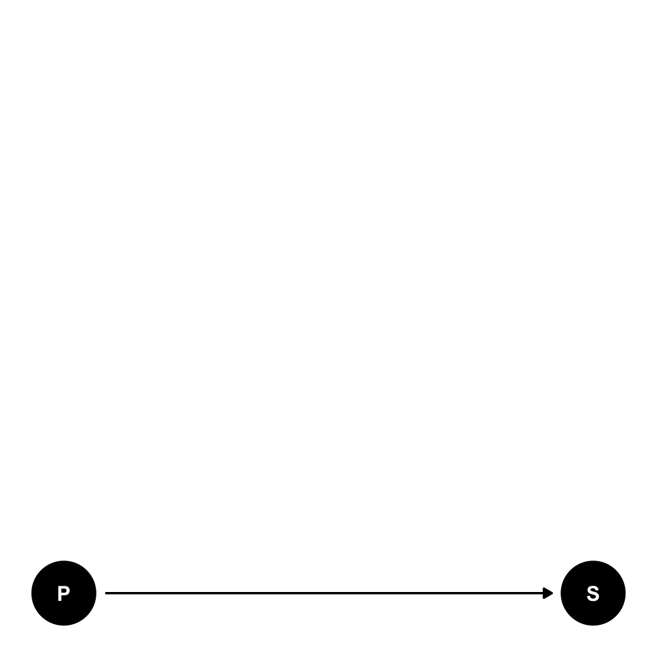
Confound: multicultural context

C = multicultural context, P = proficiency, S = code-switching. Schächinger Tenés et al. (2023)

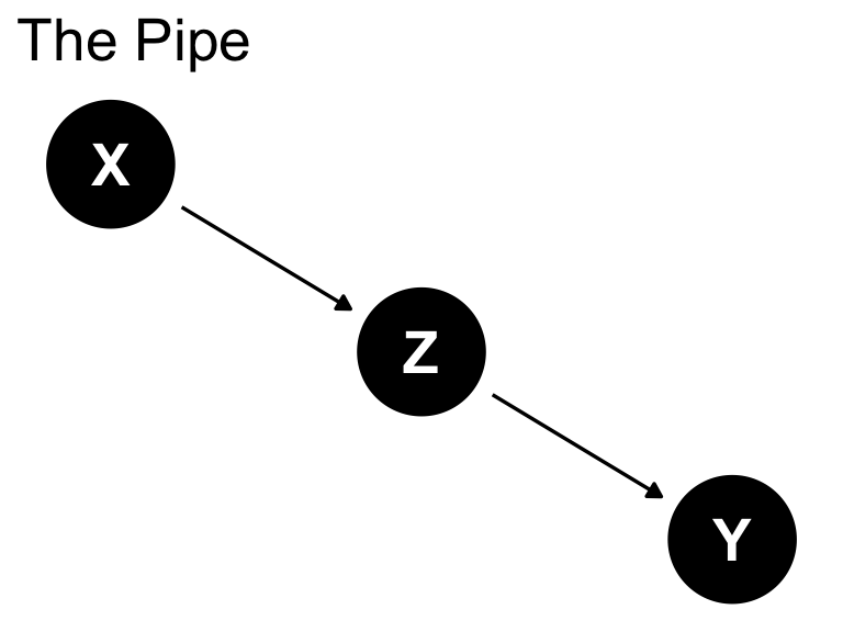
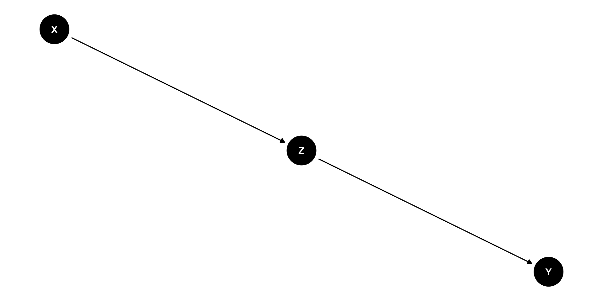
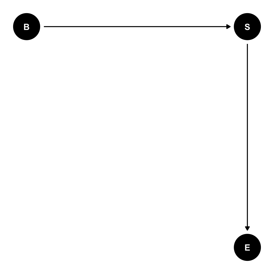
The Pipe: Z is a mediator

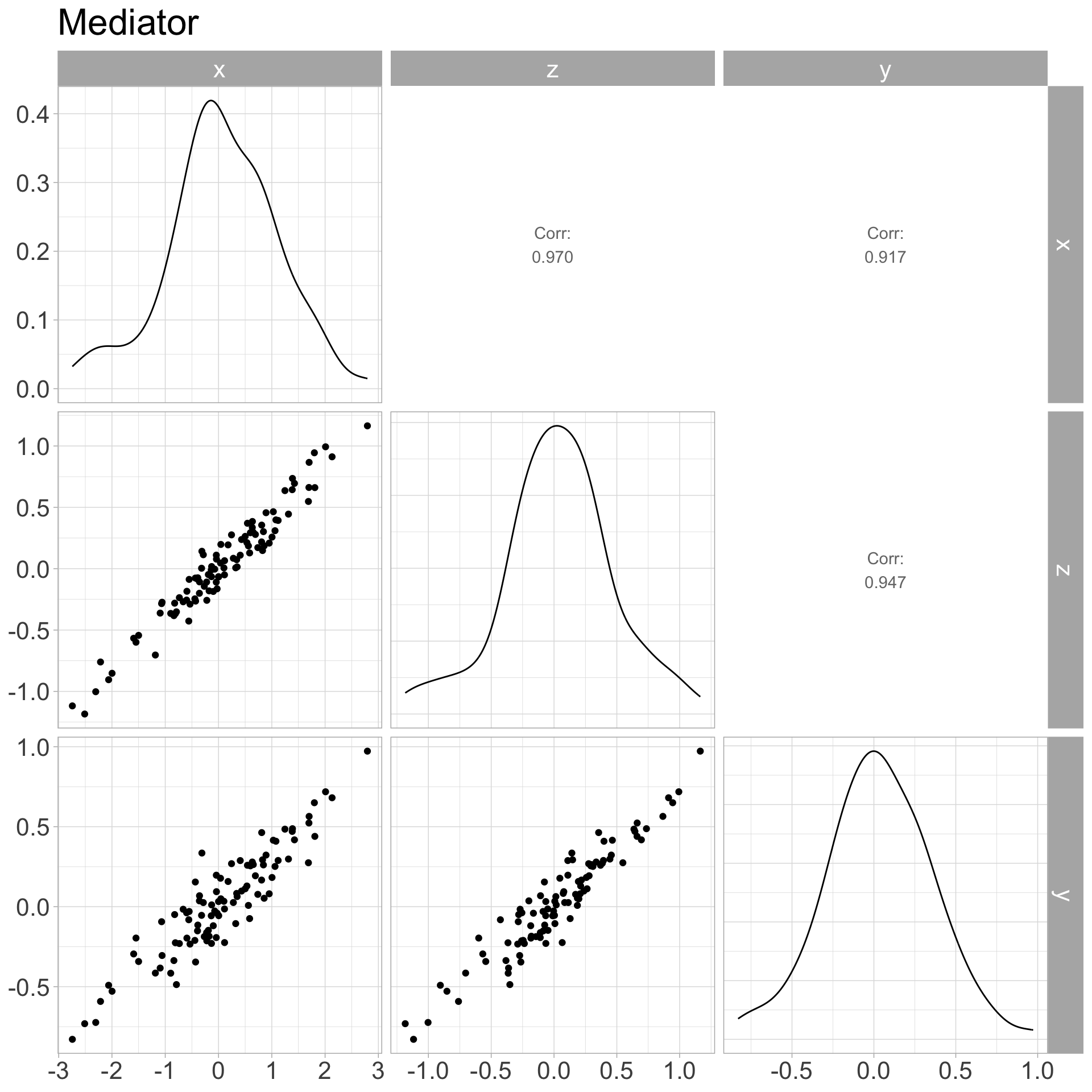
Mediator: simulate

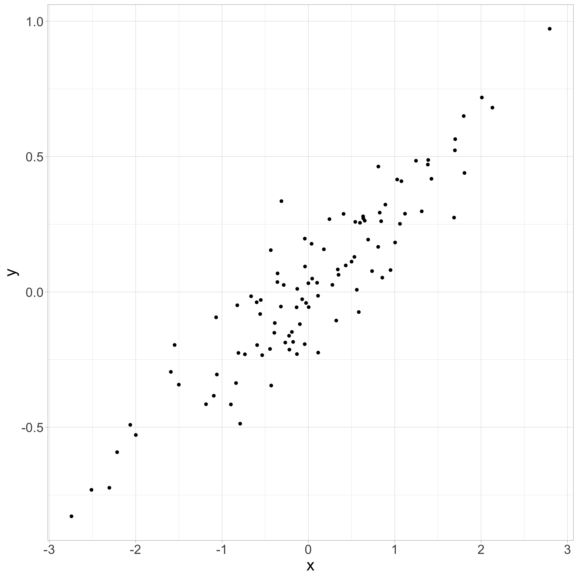
set.seed(9988)

n <- 100

x <- rnorm(n)

z <- 0.4 * x + rnorm(n, 0, 0.1)
y <- 0.7 * z + rnorm(n, 0, 0.1)

Mediator: bilingualism and executive function

B = bilingualism, E = executive function. Paap (2014)

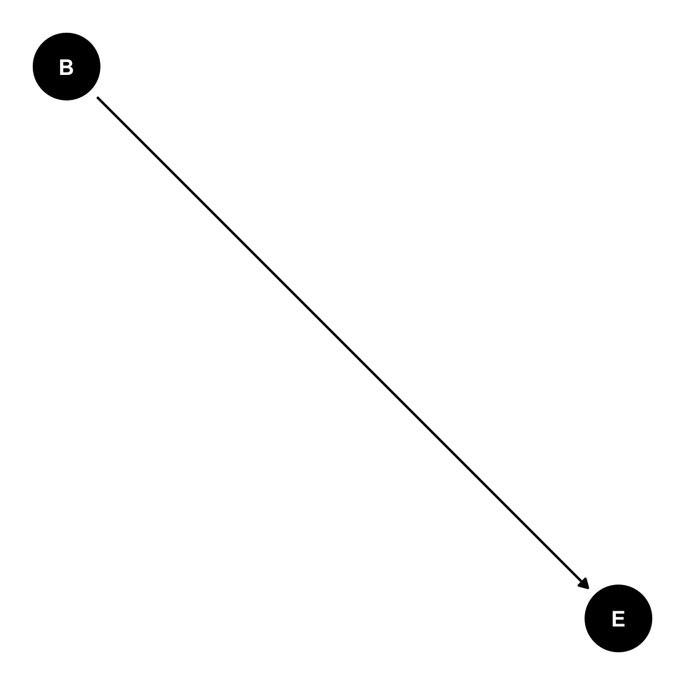
Mediator: code-switching

B = bilingualism, S = code-switching, E = executive function. Paap (2014)

Confound vs Mediator

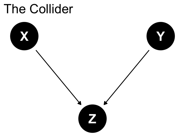
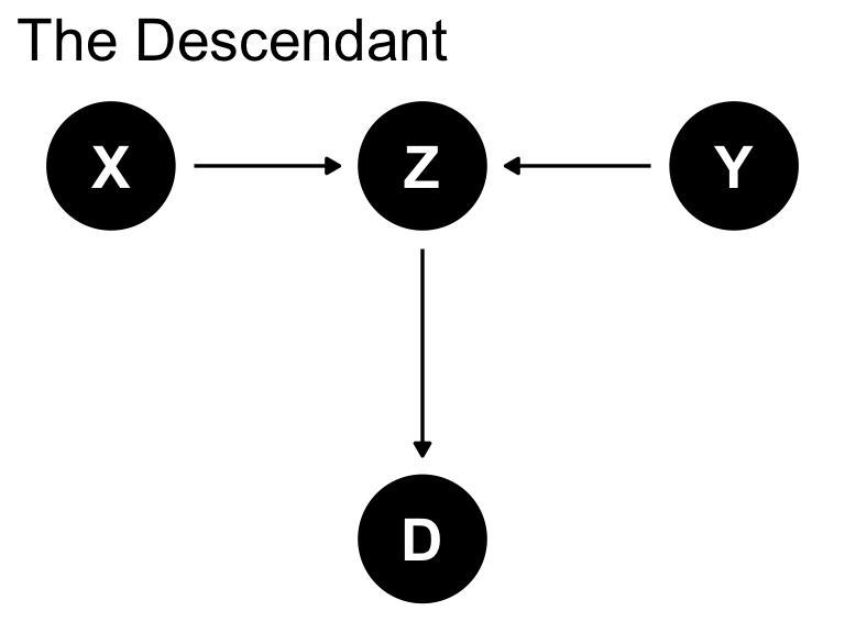
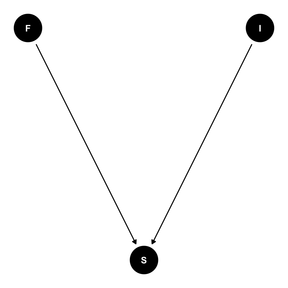
The Collider: Z is collider

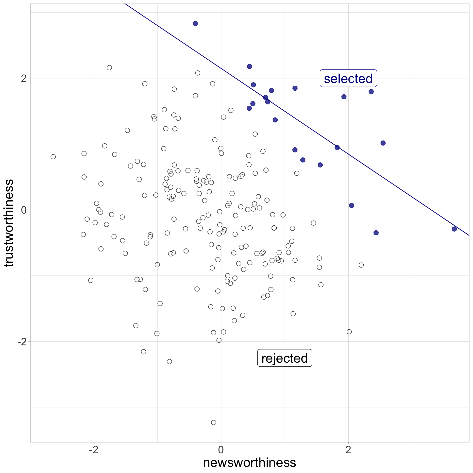
Collider: newsworthiness and trustworthiness

N = newsworthiness, T = trustworthiness, S = selected for funding. McElreath (2020)

Collider: simulate

# Adapted from https://solomon.quarto.pub/sr2/06.html#overthinking-simulated-science-distortion.
# Example from McElreath *Statistical Rethinking* (2nd ed).

set.seed(1914)

n <- 200  # Number of grant proposals
p <- 0.1  # Proportion to select

# Uncorrelated newsworthiness and trustworthiness
coll <- tibble(
  newsworthiness = rnorm(n, mean = 0, sd = 1),
  trustworthiness = rnorm(n, mean = 0, sd = 1)
) |> 
  # total_score
  mutate(total_score = newsworthiness + trustworthiness) |> 
  # Select top 10% of combined scores
  mutate(selected = ifelse(total_score >= quantile(total_score, 1 - p), TRUE, FALSE))

Collider: simulate (plot)

Collider: verb frequency and irregularity

F = frequency, I = irregularity. Wu et al. (2019)

Collider: verb saliency

F = frequency, S = saliency, I = irregularity. Wu et al. (2019)

Regression for causation

Photo by Patrick Robert Doyle on Unsplash

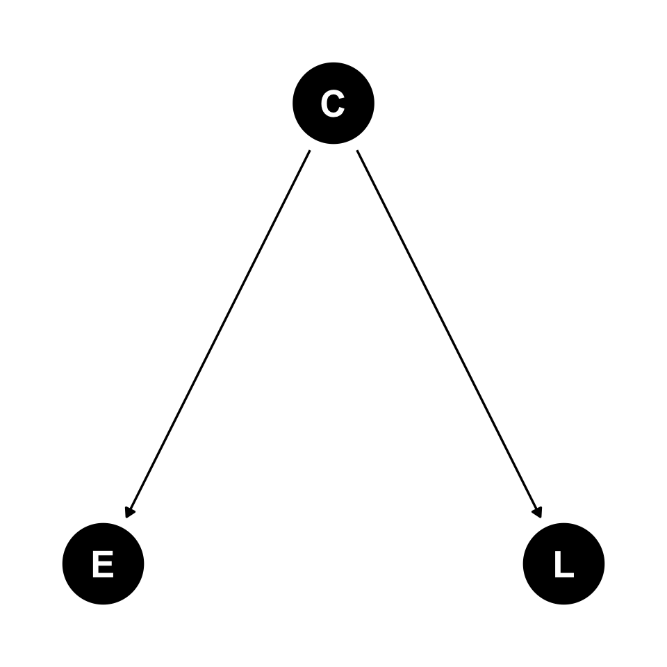
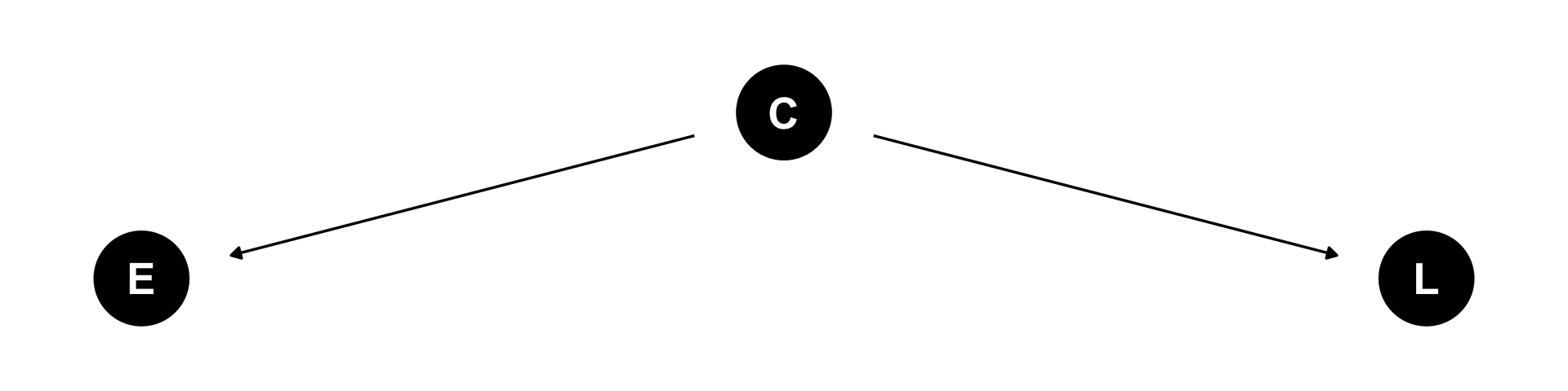
Colonial history (confound)

C = colonial history, E = economic development, L = language endangerment.

Colonial history: simulate

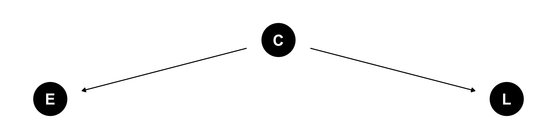
set.seed(9988)

n <- 100

C <- rnorm(n)

E <- 0.4 * C + rnorm(n, 0, 0.1)
L <- 0.7 * C + rnorm(n, 0, 0.1)

col_df <- tibble(C, E, L)

C = colonial history, E = economic development, L = language endangerment.

Colonial history: regression

conf_lm_1 <- lm(L ~ E, data = col_df)

            Estimate Std. Error
(Intercept)    0.004      0.021
E              1.599      0.047

conf_lm_2 <- lm(L ~ E + C, data = col_df)

            Estimate Std. Error
(Intercept)    0.008      0.011
E              0.019      0.098
C              0.690      0.042

C = colonial history, E = economic development, L = language endangerment.

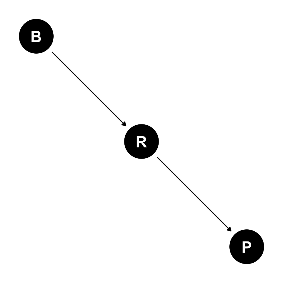
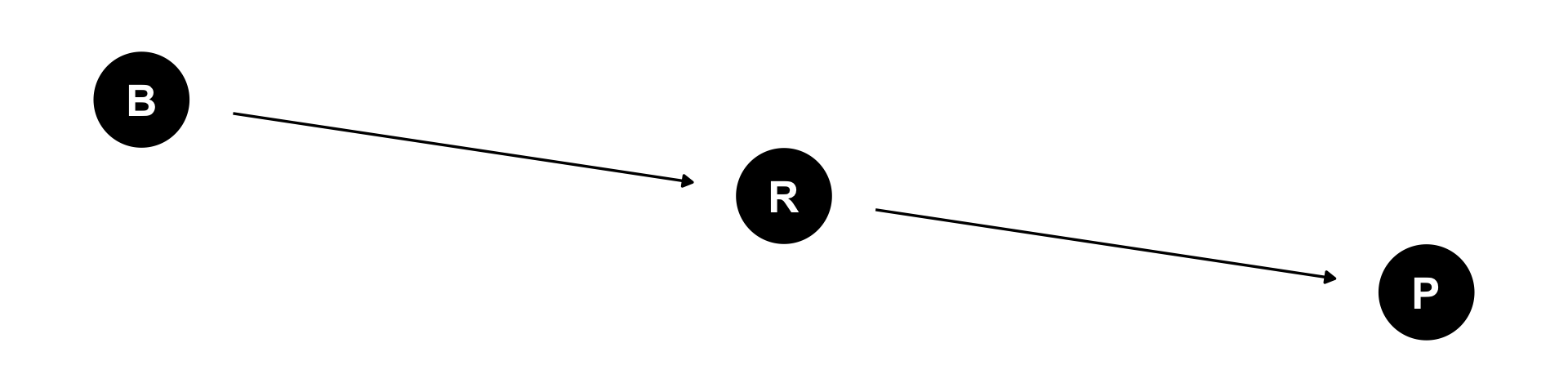
Plant reliance (mediator)

B = biodiversity, R = reliance on plants, P = number of plant names.

Plant reliance: simulate

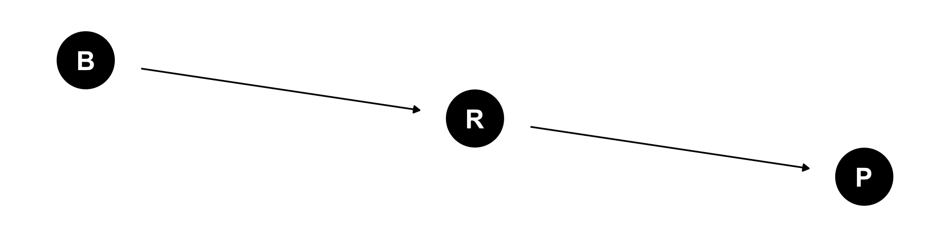
set.seed(9988)

n <- 100

B <- rnorm(n)

R <- 0.4 * B + rnorm(n, 0, 0.1)
P <- 0.7 * R + rnorm(n, 0, 0.1)

pla_df <- tibble(B, R, P)

Plant reliance: regression

med_lm_1 <- lm(P ~ B, data = pla_df)

            Estimate Std. Error
(Intercept)    0.012      0.013
B              0.286      0.013

med_lm_2 <- lm(P ~ B + R, data = pla_df)

            Estimate Std. Error
(Intercept)    0.008      0.011
B             -0.010      0.042
R              0.719      0.098

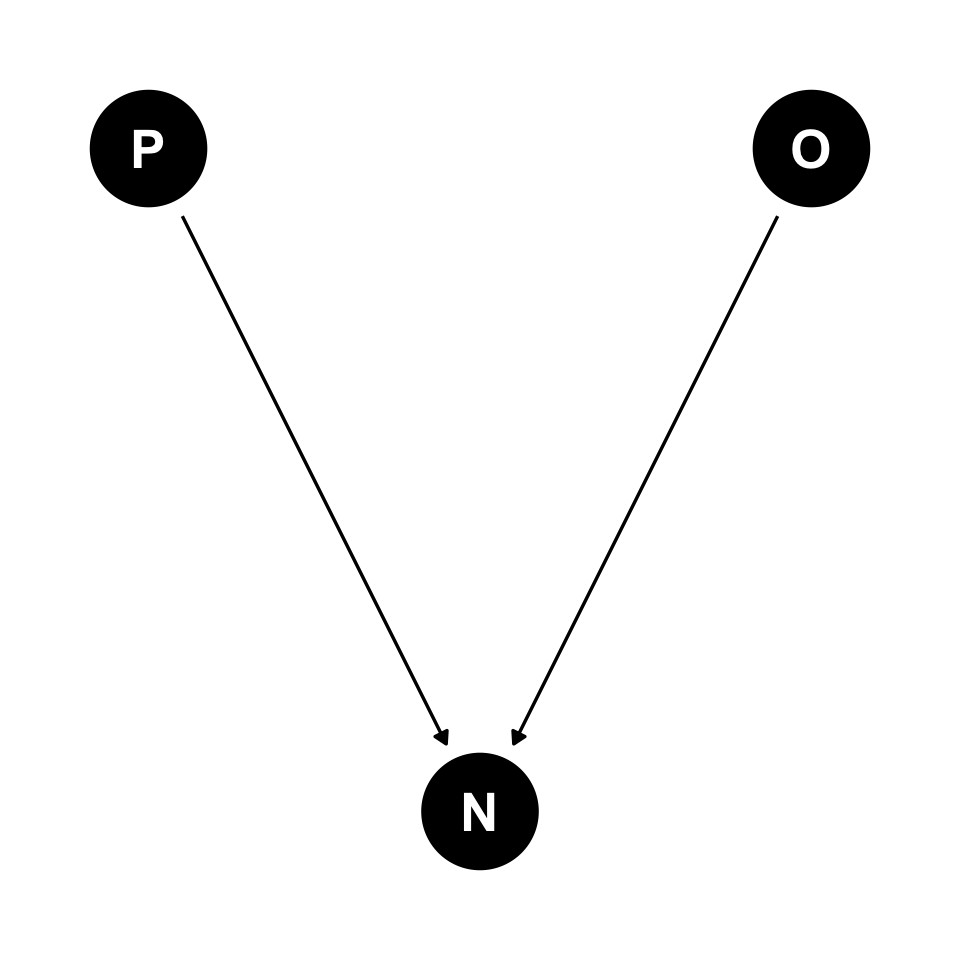
Number of learners (collider)

P = prestige, O = official, N = number of learners.

Number of learners: simulate

set.seed(9988)

n <- 100

learn_df <- tibble(
  prestige = rnorm(n, mean = 0, sd = 1),
  official = rbinom(n, size = 1, prob = 0.3)
) |> 
  mutate(
    n_learn = 0.4 * prestige + 0.2 * official +
      rnorm(n, mean = 0, sd = 1)
  )

P = prestige, O = official, N = number of learners.

Number of learners: regression

coll_lm_1 <- lm(
  prestige ~ official,
  data = learn_df
)

            Estimate Std. Error
(Intercept)    0.064      0.129
official       0.004      0.222

coll_lm_2 <- lm(
  prestige ~ official + n_learn,
  data = learn_df
)

            Estimate Std. Error
(Intercept)    0.070      0.118
official      -0.138      0.205
n_learn        0.384      0.086

P = prestige, O = official, N = number of learners.

Conditional independences

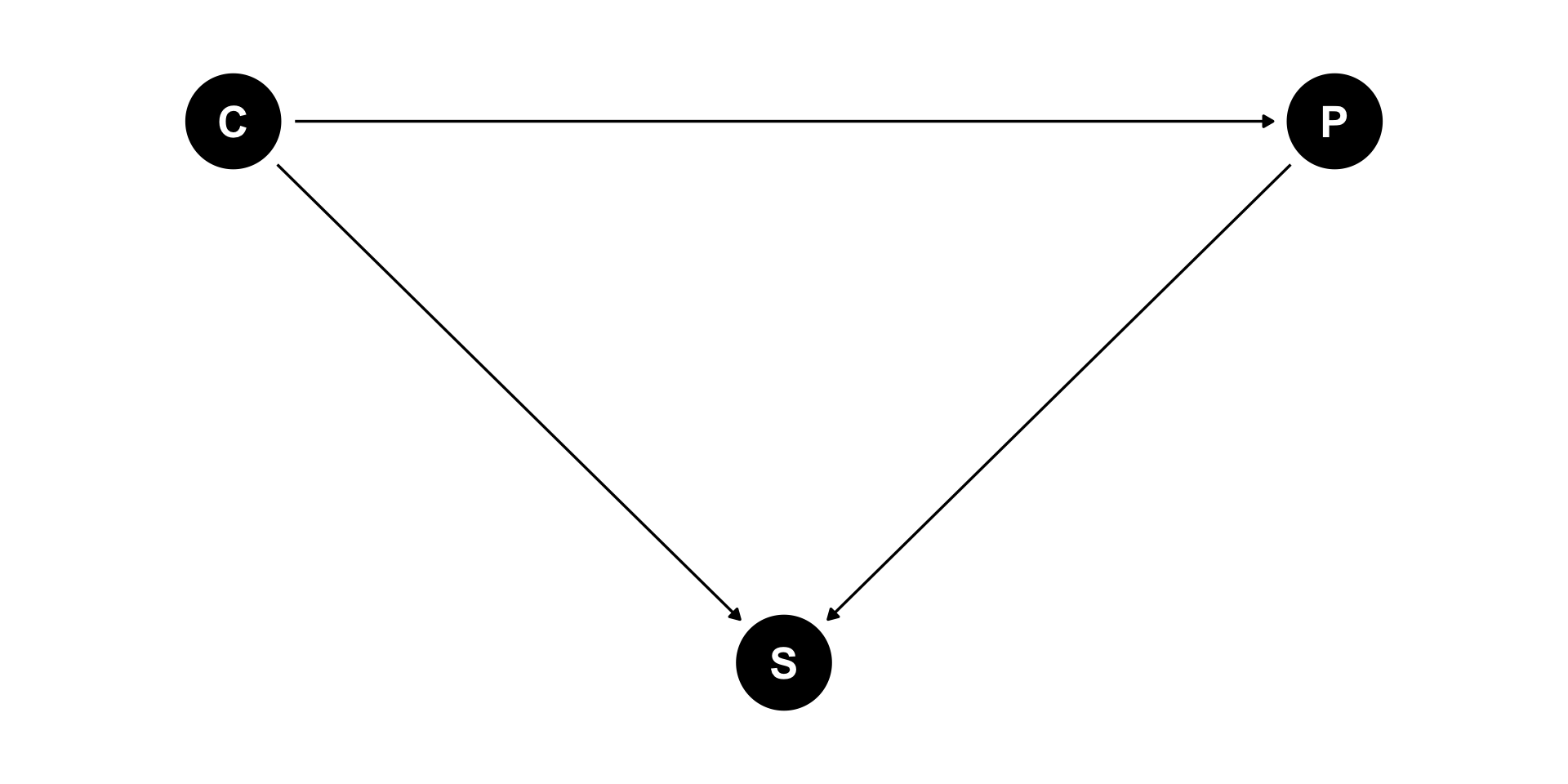
\(P \not\!\perp\!\!\!\perp C\)

\(S \not\!\perp\!\!\!\perp C\)

\(S \not\!\perp\!\!\!\perp P\)

\(\perp\!\!\!\perp\) = “independent”

\(\not\!\perp\!\!\!\perp\) = “not independent”

C = multicultural context, P = proficiency, S = code-switching. Schächinger Tenés et al. (2023)

Conditional independences

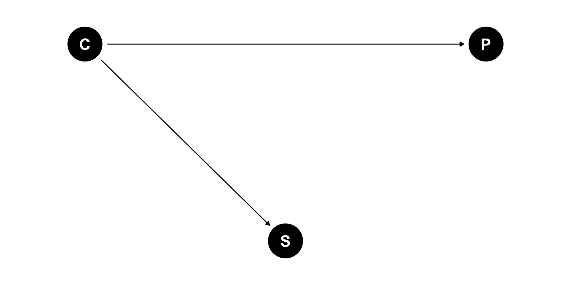
\(P \not\!\perp\!\!\!\perp C\)

\(S \not\!\perp\!\!\!\perp C\)

\(S \perp\!\!\!\perp P | C\)

P is not independent of C

S is not independent of C

S is independent of P, conditional on C

C = multicultural context, P = proficiency, S = code-switching. Schächinger Tenés et al. (2023)

Causal paths

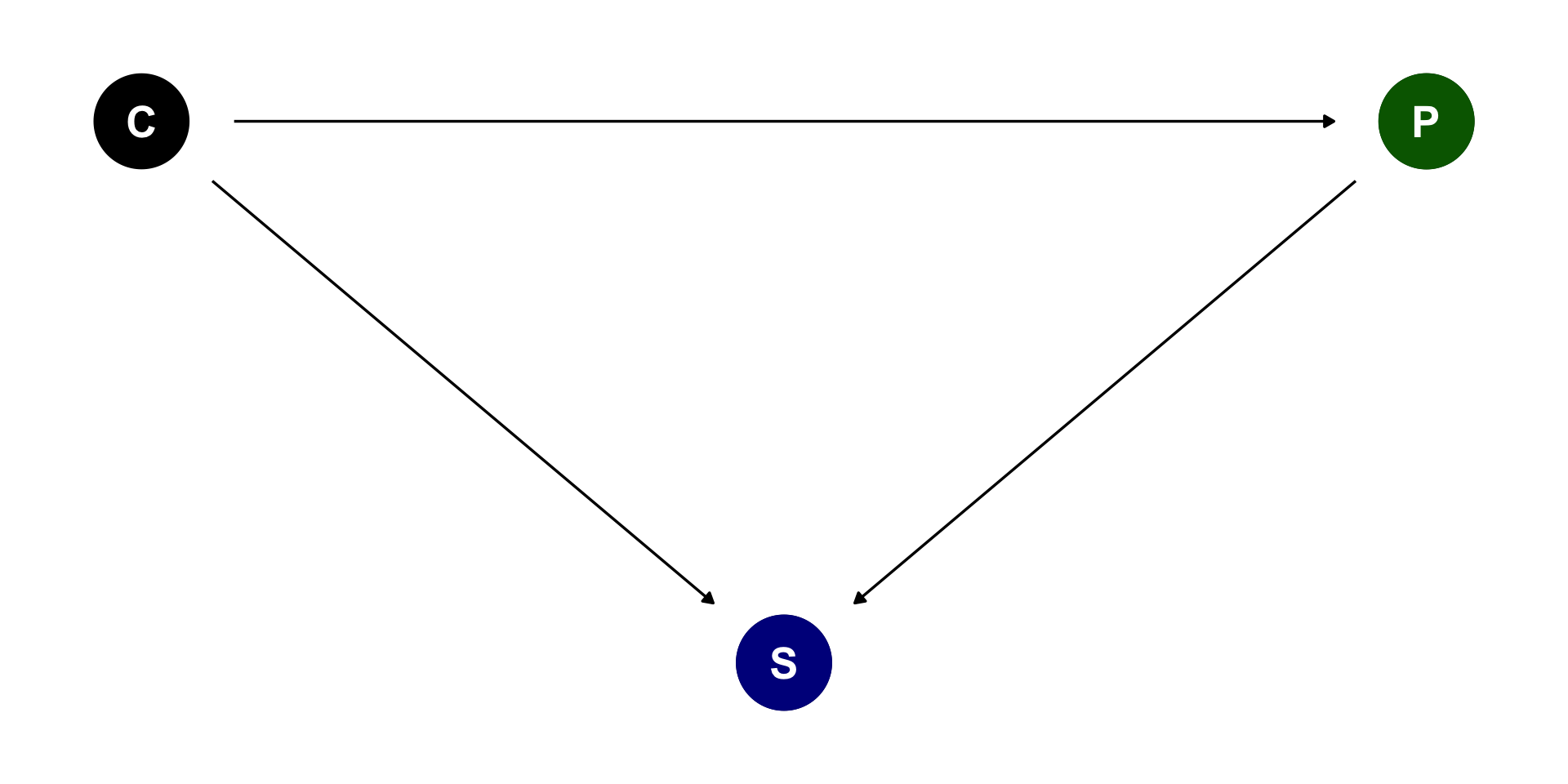
\(P \rightarrow S\)

\(P \leftarrow C \rightarrow S\)

Causal paths

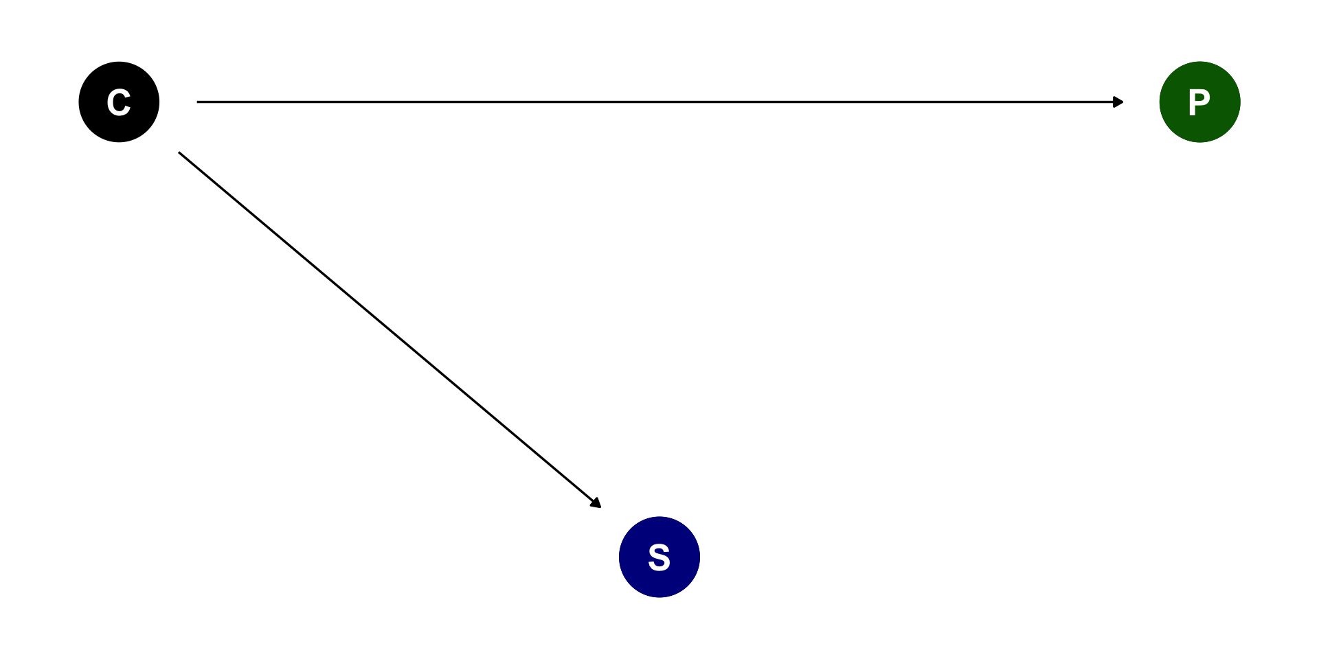
\(S \leftarrow C \rightarrow p\)

Shutting the backdoor

Backdoor recipe

1. List all of the paths connecting X (the potential cause of interest) and Y (the outcome).

2. Classify each path by whether it is open or closed. A path is open unless it contains a collider.

3. Classify each path by whether it is a backdoor path. A backdoor path has an arrow entering X.

4. If there are any open backdoor paths, decide which variable(s) to condition on to close it (if possible).

Workplace and use of prestige variable

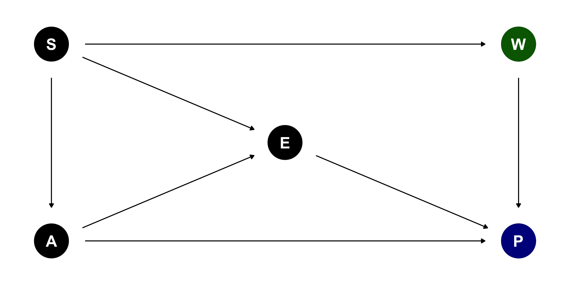
Path	Open	Backdoor
\(W \rightarrow P\)	yes	no
\(W \leftarrow S \rightarrow A \rightarrow E \rightarrow P\)	yes	yes
\(W \leftarrow S \rightarrow A \rightarrow P\)	yes	yes
\(W \leftarrow S \rightarrow E \rightarrow P\)	yes	yes
\(W \leftarrow S \rightarrow E \leftarrow A \rightarrow P\)	no	yes

S = socio-economic status, A = exposure age, E = exposure degree, W = workplace style, P = use of prestige.

Workplace and use of prestige: adjustment sets

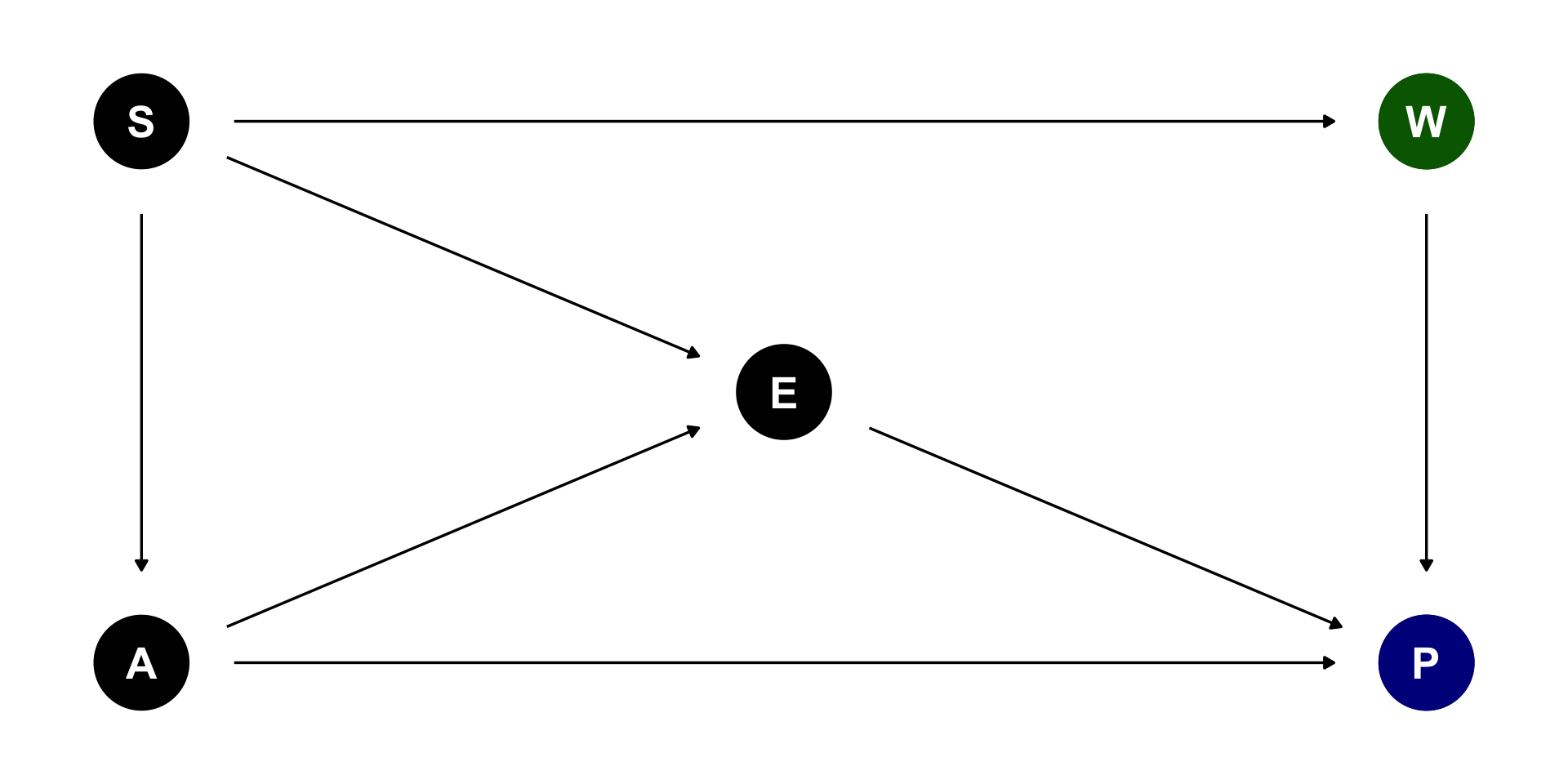
A, E

S

lm(P ~ W + S)

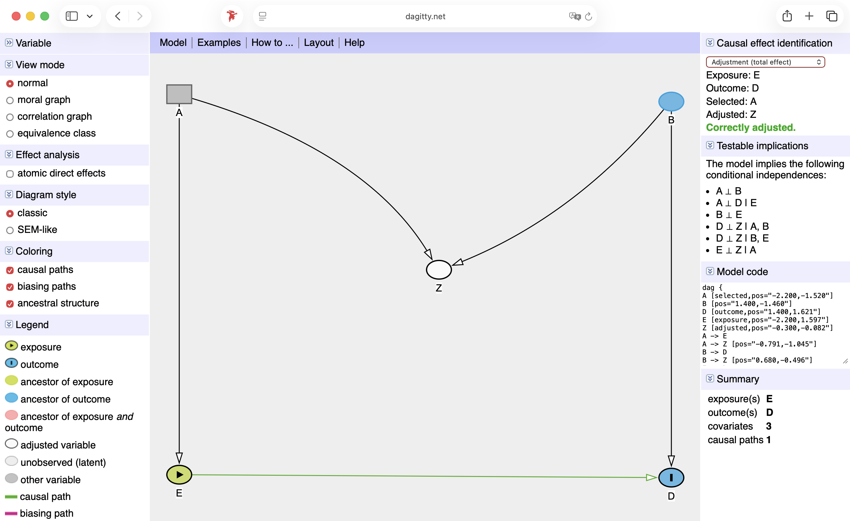
Dagitty

Limitations

It assumes DAG is correct.

Adjustment variables should be observable.

Complex systems require dynamic system modelling.

Tick icons created by Roundicons - Flaticon Unknown icons created by Freepik - Flaticon Strange icons created by Jagat Icon - Flaticon

Summary

Correlation is causation (if you use causal inference).

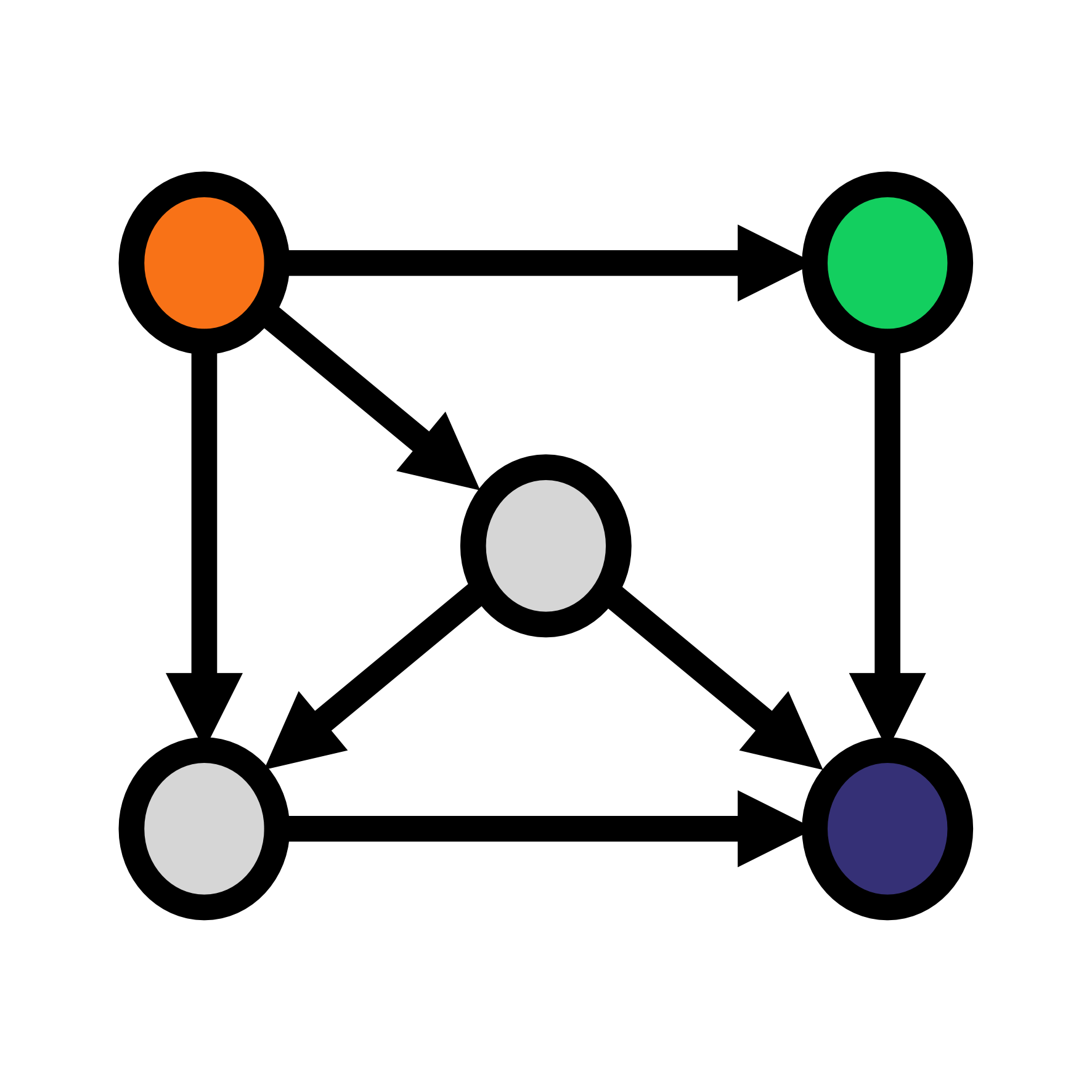
Directed Acyclic Graphs (DAGs).

Choose your covariates carefully.

References

McElreath, Richard. 2020. Statistical Rethinking: A Bayesian Course with Examples in R and Stan. Second edition. Chapman & Hall/CRC Texts in Statistical Science Series. CRC Press.

Paap, Kenneth R. 2014. “Bilingual Advantages in Executive Functioning: Problems in Convergent Validity, Discriminant Validity, and the Identification of the Theoretical Constructs.” Frontiers in Psychology 5. https://doi.org/10.3389/fpsyg.2014.00962.

Pander Maat, Henk. 2017. “Zinslengte en zinscomplexiteit: Een corpusbenadering.” Tijdschrift voor Taalbeheersing 39 (3): 297–328. https://doi.org/10.5117/TVT2017.3.PAND.

Schächinger Tenés, L. T., J. C. Weiner-Bühler, L. Volpin, A. Grob, K. Skoruppa, and R. K. Segerer. 2023. “Language Proficiency Predictors of Code-Switching Behavior in Dual-Language-Learning Children.” Bilingualism: Language and Cognition 26 (5): 942–58. https://doi.org/10.1017/S1366728923000081.

Wu, Shijie, Ryan Cotterell, and Timothy O’Donnell. 2019. “Morphological Irregularity Correlates with Frequency.” Proceedings of the 57th Annual Meeting of the Association for Computational Linguistics (Florence, Italy), 5117–26. https://doi.org/10.18653/v1/P19-1505.