05 - Poisson and ordinal regression models for count variables and likert scales

Stefano Coretta

Summary

Gaussian for Gaussian variables (very rare).
Log-normal for outcome variables that can take only positive (real) values.
Bernoulli for binary outcome variables.

Other common types of outcome variables:

Count data: Poisson and negative binomial models.
Likert scales: Ordinal models.

Counts of infants’ gestures

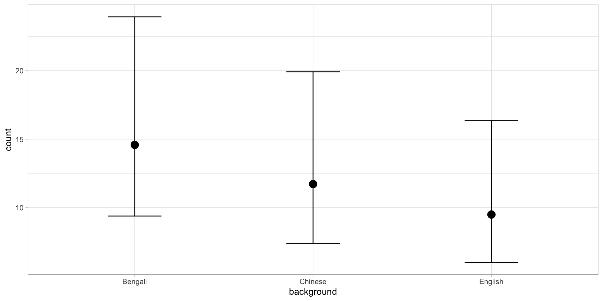
gestures <- read_csv("data/cameron2020/gestures.csv")
gestures_count <- gestures |>
  filter(months == 11) |> 
  summarise(
    count = sum(count, na.rm = TRUE),
    .by = c(background, dyad)
  )

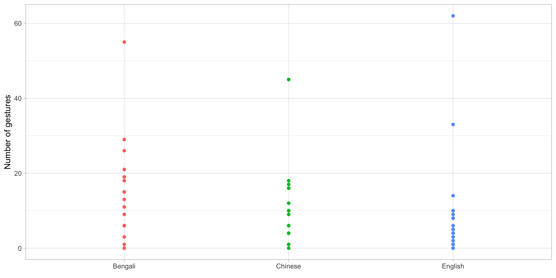
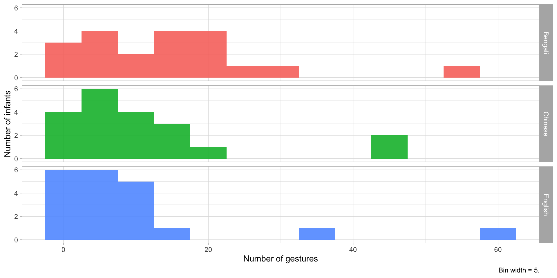
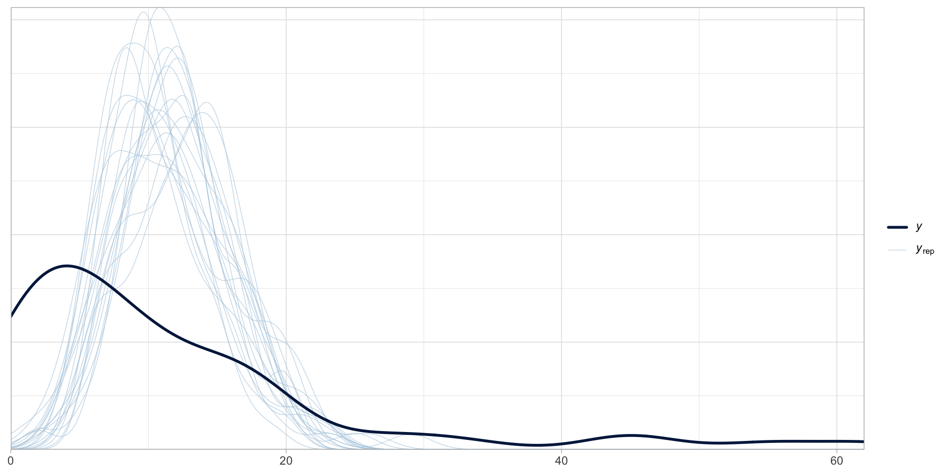
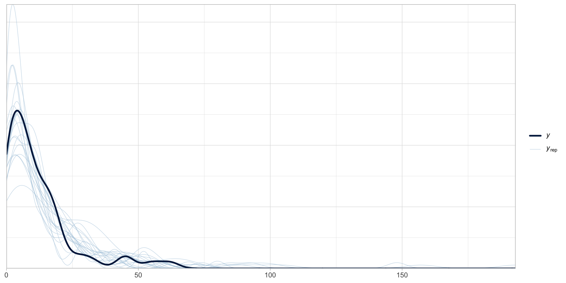
gestures_count

# A tibble: 60 × 3
   background dyad  count
   <chr>      <chr> <dbl>
 1 Bengali    b01       9
 2 Bengali    b02      18
 3 Bengali    b03      15
 4 Bengali    b04      21
 5 Bengali    b05      13
 6 Bengali    b06       6
 7 Bengali    b07       6
 8 Bengali    b08      19
 9 Bengali    b09       6
10 Bengali    b10       1
# ℹ 50 more rows

Infants’ gestures

Figure 1: Number of gestures by infant and group.

Infants’ gestures: histogram

Figure 2: Histogram of number of gestures by group.

Poisson regression: code

gest_pois <- brm(
  count ~ 0 + background,
  family = poisson,
  data = gestures_count,
  cores = 4,
  seed = 8712,
  file = "data/cache/gest_pois"
)

Poisson regression: posterior predictive check

pp_check(gest_pois, ndraws = 20)

Figure 3: Posterior predictive check plot of gest_pois.

Negative binomial regression: code

gest_negb <- brm(
  count ~ 0 + background,
  family = negbinomial,
  data = gestures_count,
  cores = 4,
  seed = 8258,
  file = "data/cache/gest_negb"
)

Negative binomial: posterior predictive check

pp_check(gest_negb, ndraws = 20)

Figure 4: Posterior predictive check of gest_negb.

Negative binomial: predicted counts

conditional_effects(gest_negb)

Figure 5: Predicted counts of gestures by background.

Posterior draws

gest_negb_draws <- as_draws_df(gest_negb)

gest_negb_draws

# A draws_df: 1000 iterations, 4 chains, and 6 variables
   b_backgroundBengali b_backgroundChinese b_backgroundEnglish shape lprior
1                  2.6                 2.3                 2.3  1.05   -1.6
2                  2.7                 2.5                 2.4  0.97   -1.5
3                  2.6                 2.3                 2.5  0.77   -1.3
4                  2.6                 2.6                 2.0  1.07   -1.6
5                  2.8                 2.1                 2.2  1.70   -2.2
6                  2.5                 2.3                 2.8  1.39   -2.0
7                  2.4                 2.3                 2.7  1.29   -1.9
8                  2.5                 2.7                 2.2  0.83   -1.4
9                  2.7                 2.1                 2.7  0.97   -1.5
10                 2.7                 2.8                 2.5  0.81   -1.4
   lp__
1  -211
2  -211
3  -212
4  -212
5  -218
6  -217
7  -215
8  -212
9  -214
10 -213
# ... with 3990 more draws
# ... hidden reserved variables {'.chain', '.iteration', '.draw'}

Predicted counts

gest_negb_draws <- gest_negb_draws |> 
  mutate(
    Bengali = exp(b_backgroundBengali),
    Chinese = exp(b_backgroundChinese),
    English = exp(b_backgroundEnglish)
  )

gest_negb_draws |> select(Bengali:English)

# A tibble: 4,000 × 3
   Bengali Chinese English
     <dbl>   <dbl>   <dbl>
 1    13.0    9.86    9.83
 2    14.4   11.8    10.5 
 3    14.0    9.74   12.5 
 4    13.9   13.7     7.16
 5    17.1    8.31    9.35
 6    12.2    9.90   16.3 
 7    11.5   10.3    14.3 
 8    12.4   15.1     8.72
 9    14.7    8.29   15.0 
10    15.1   16.8    11.9 
# ℹ 3,990 more rows

Credible intervals: counts

gest_negb_draws |> 
  select(Bengali:English) |> 
  pivot_longer(Bengali:English, names_to = "coef", values_to = "est") |> 
  group_by(coef) |> 
  summarise(
    ci_lo = round(quantile2(est, probs = 0.025)),
    ci_hi = round(quantile2(est, probs = 0.975))
  )

# A tibble: 3 × 3
  coef    ci_lo ci_hi
  <chr>   <dbl> <dbl>
1 Bengali     9    24
2 Chinese     7    20
3 English     6    16

Summary I

Count data (like the number of infants’ gestures, or number of occurrences in a corpus) can be modelled with a Poisson distribution.
If the data has over-dispersion, the negative binomial distribution might be better.
The model estimates are in logged counts. Use exp() to convert them back to counts.

Likert scales

emilianto <- readRDS("data/hampton2023/emilianto_attitude.rds")

emilian <- emilianto |> 
  filter(language == "Emilian")

emilian |> select(comprehend, speak, commuter, age)

# A tibble: 434 × 4
   comprehend speak commuter   age
   <ord>      <ord> <chr>    <dbl>
 1 VG         VG    Sí          57
 2 G          50/50 No          20
 3 VG         VG    No          50
 4 50/50      NO    No          25
 5 VG         VG    No          65
 6 VG         VG    No          56
 7 VG         VG    No          62
 8 VG         VG    No          65
 9 VG         VG    No          63
10 VG         G     No          61
# ℹ 424 more rows

An ordinal model of comprehension: code

compr_ord <- brm(
  comprehend ~ cs(commuter),
  family = acat(link = "probit"),
  data = emilian,
  cores = 4,
  seed = 1523,
  file = "data/cache/compr_ord"
)

Predicted probability of each

conditional_effects(compr_ord, categorical = TRUE)

Figure 6: Predicted probability of comprehension levels by commuter status.

An ordinal model of speaking proficiency: code

speak_ord <- brm(
  speak ~ age,
  family = acat(link = "probit"),
  data = emilian,
  cores = 4,
  seed = 1523,
  file = "data/cache/speak_ord"
)

Predicted probability of speaking proficiency

conditional_effects(speak_ord, categorical = TRUE)

Figure 7: Predicted probability of speaking proficiency levels by age.

Summary II

Likert scale data can be modelled with a an ordinal distribution.
Ordinal models estimate the probability of each level in the scale.