04 - Bernoulli models for binary outcomes

Stefano Coretta

MALD: accuracy

• Accuracy of responses: correctly or incorrectly recognised the word type (real or nonce-word).

• Let’s model the effect of phonetic distance on accuracy.

• Accuracy is a binary variable.

• With binary variables we model the probability of one of the two levels. Here, correct.

• The probability of one level of a binary variable follows a Bernoulli distribution.

Bernoulli model

\[ p(correct) \sim Bernoulli(p) \]

• But… probabilities are bounded between 0 and 1.

• For variables that can only have positive real numbers, we used the logarithmic function (log-normal models).

• With probabilities, we can use the logistic function.

• The logistic (or logit) function converts probabilities to log-odds (qlogis() in R).

Logistic function

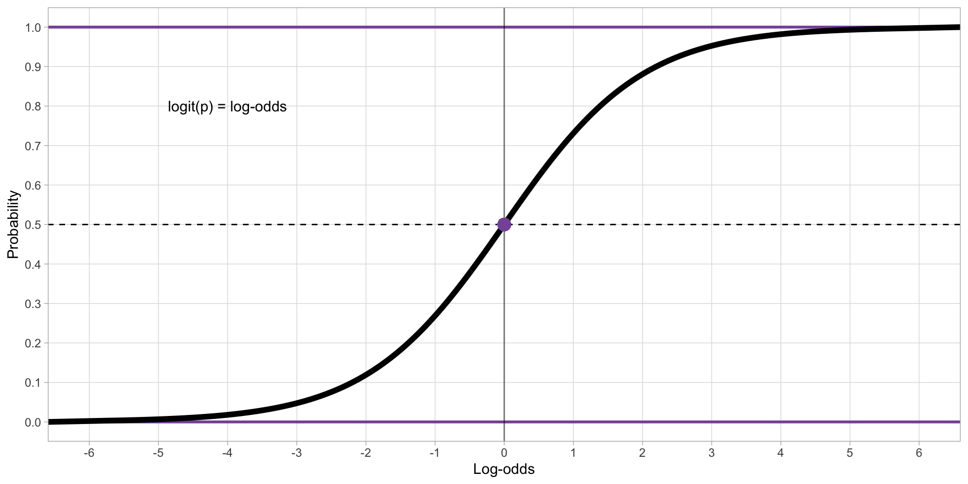
Figure 1: Correspondence between log-odds and probabilities.

Bernoulli (regression) models

• Bernoulli models use the logistic function to treat probabilities as if they were unbounded.

• The model’s estimates are in log-odds.

• Log-odds can be converted back to probabilities with the inverse logit function (plogis() in R).

• Bernoulli models are also known as binomial or logistic regression.

A Bernoulli regression of accuracy: code

acc_bern <- brm(
  ACC ~ 1 + PhonLev,
  family = bernoulli,
  data = mald,
  cores = 4,
  seed = 8230,
  file = "data/cache/acc_bern"
)

A Bernoulli regression of accuracy: predicted accuracy

conditional_effects(acc_bern)

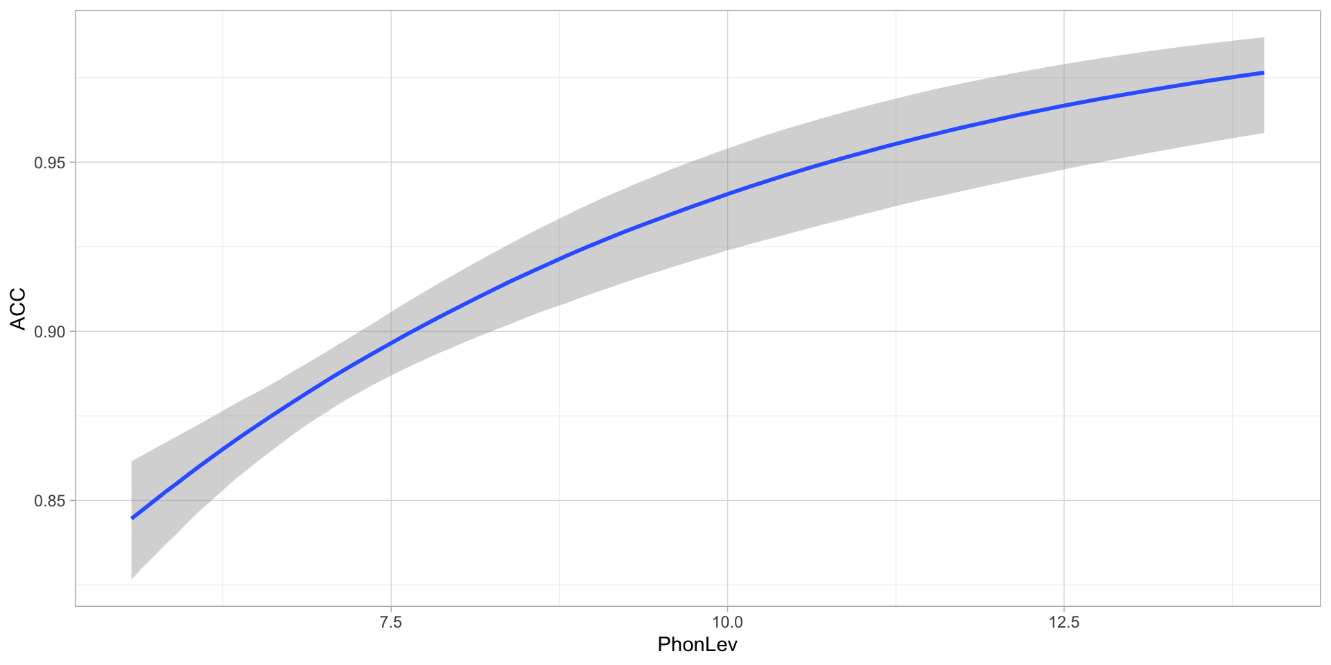
Figure 2: Predicted accuracy based on phonetic distance.

Brentari 2024: Lengua de Señas Nicaragüense (LSN)

brentari2024 <- read_csv("data/brentari2024/verb_org.csv")

brentari2024

# A tibble: 630 × 6
   Group    Participant Object   Number Agency   Num_Predicates
   <chr>          <dbl> <chr>    <chr>  <chr>    <chr>         
 1 homesign           1 book     single agent    multiple      
 2 homesign           1 book     single agent    multiple      
 3 homesign           1 book     plural no_agent multiple      
 4 homesign           1 coin     single agent    single        
 5 homesign           1 coin     plural no_agent single        
 6 homesign           1 coin     single no_agent single        
 7 homesign           1 coin     single no_agent multiple      
 8 homesign           1 lollipop single agent    single        
 9 homesign           1 lollipop single agent    single        
10 homesign           1 lollipop plural no_agent single        
# ℹ 620 more rows

Brentari 2024

brentari2024 |> 
  ggplot(aes(Group, fill = Num_Predicates)) +
  geom_bar(position = "fill") +
  labs(y = "Proportion")

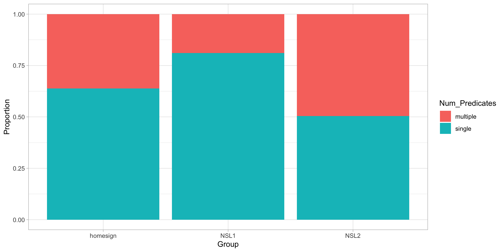
Figure 3: Proportion of predicate type by group.

A Bernoulli model of predicate type

\[ \begin{align} pred_i & \sim Bernoulli(p_i)\\ logit(p_i) & = \beta_1 \cdot G_{\text{HS}[i]} + \beta_2 \cdot G_{\text{NSL1}[i]} + \beta_3 \cdot G_{\text{NSL2}[i]} \end{align} \]

• logit(p) indicates a logit function is used (so the estimates are in log-odds).

• \(G_{\text{HS}[i]}, G_{\text{NSL1}[i]},G_{\text{NSL2}[i]}\) are indicator variables, a way of including categorical predictors in a regression model.

Indicator variables

	\(G_{\text{HS}}\)	\(G_{\text{NSL1}}\)	\(G_{\text{NSL2}}\)
Homesign	1	0	0
NSL1	0	1	0
NSL2	0	0	1

\[ \begin{align} logit(p_i) & = \beta_1 \cdot G_{\text{HS}[i]} + \beta_2 \cdot G_{\text{NSL1}[i]} + \beta_3 \cdot G_{\text{NSL2}[i]}\\ \text{homesign, } logit(p_i) & = \beta_1 \cdot 1 + \beta_2 \cdot 0 + \beta_3 \cdot 0\\ & = \beta_1\\ \text{NSL1, } logit(p_i) & = \beta_1 \cdot 0 + \beta_2 \cdot 1 + \beta_3 \cdot 0\\ & = \beta_2\\ \text{NSL2, } logit(p_i) & = \beta_1 \cdot 0 + \beta_2 \cdot 0 + \beta_3 \cdot 1\\ & = \beta_3\\ \end{align} \]

Indicator variables

• Note that indicator variables are dealt with by brms under the hood.

• We talk about them to understand how the model is set up.

• The model will estimate the probability \(p\) for each group.

• But… the probability of what?

Prepare data

table(brentari2024$Num_Predicates)

multiple   single 
     215      415 

brentari2024 <- brentari2024 |> 
  mutate(
    Pred_Type = factor(Num_Predicates, levels = c("single", "multiple"))
  )

table(brentari2024$Pred_Type)

  single multiple 
     415      215 

• The model will estimate the probability \(p\) of finding a multiple predicate, depending on group.

A Bernoulli model of predicate type: suppress the intercept

v1_duration ~ 1 + speech_rate_c

• 1 stands for “intercept”. The model has an intercept and a slope.

Pred_Type ~ 0 + Group

• 0 stands for “suppress the overall intercept”. The model estimates one “intercept” per level.

A Bernoulli model of predicate type: code

pred_bern <- brm(
  Pred_Type ~ 0 + Group,
  family = bernoulli,
  data = brentari2024,
  cores = 4,
  seed = 3218,
  file = "data/cache/pred_bern"
)

A Bernoulli model of predicate type: summary

summary(pred_bern)

 Family: bernoulli 
  Links: mu = logit 
Formula: Pred_Type ~ 0 + Group 
   Data: brentari2024 (Number of observations: 630) 
  Draws: 4 chains, each with iter = 2000; warmup = 1000; thin = 1;
         total post-warmup draws = 4000

Regression Coefficients:
              Estimate Est.Error l-95% CI u-95% CI Rhat Bulk_ESS Tail_ESS
Grouphomesign    -0.57      0.16    -0.87    -0.26 1.00     4384     3351
GroupNSL1        -1.46      0.17    -1.79    -1.14 1.00     4209     2946
GroupNSL2        -0.02      0.14    -0.29     0.25 1.00     3865     2727

Draws were sampled using sampling(NUTS). For each parameter, Bulk_ESS
and Tail_ESS are effective sample size measures, and Rhat is the potential
scale reduction factor on split chains (at convergence, Rhat = 1).

A Bernoulli model of predicate type: predicted probability

conditional_effects(pred_bern)

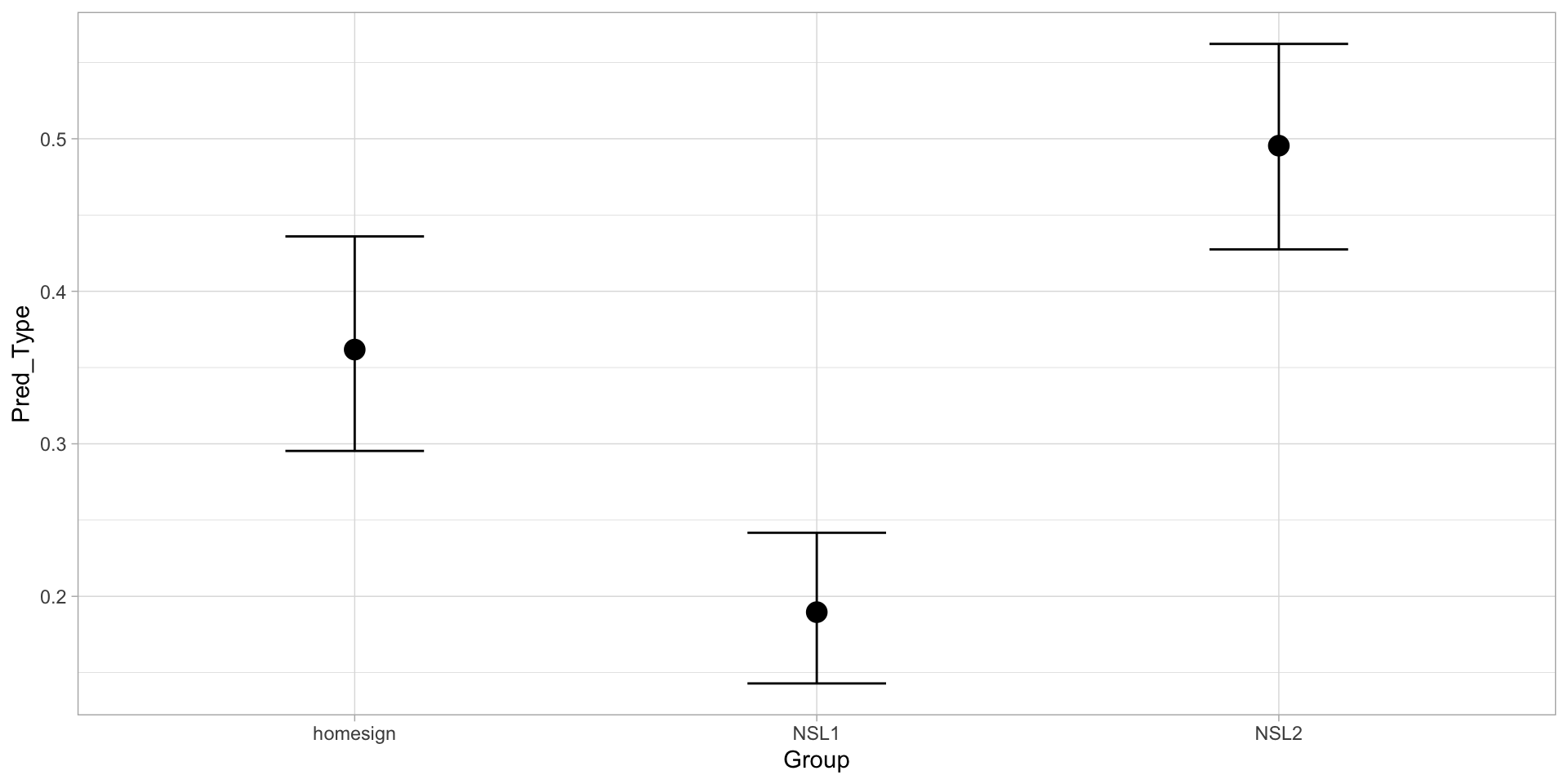
Figure 4: Predicted probability of multiple predicate by group.

Posterior draws

pred_bern_draws <- as_draws_df(pred_bern)

pred_bern_draws

# A draws_df: 1000 iterations, 4 chains, and 5 variables
   b_Grouphomesign b_GroupNSL1 b_GroupNSL2 lprior lp__
1            -0.43        -1.6      -0.112      0 -381
2            -0.17        -1.5      -0.049      0 -384
3            -0.81        -1.4      -0.205      0 -383
4            -0.52        -1.4      -0.110      0 -381
5            -0.74        -1.4      -0.175      0 -382
6            -0.21        -1.2       0.065      0 -384
7            -0.89        -1.3      -0.037      0 -383
8            -0.47        -1.3       0.095      0 -381
9            -0.56        -1.3       0.081      0 -381
10           -0.67        -1.5       0.048      0 -381
# ... with 3990 more draws
# ... hidden reserved variables {'.chain', '.iteration', '.draw'}

Credible intervals: log-odds

library(posterior)

pred_bern_draws |> 
  pivot_longer(b_Grouphomesign:b_GroupNSL2, names_to = "coef", values_to = "est") |> 
  group_by(coef) |> 
  summarise(
    ci_lo = quantile2(est, probs = 0.025),
    ci_hi = quantile2(est, probs = 0.975)
  )

# A tibble: 3 × 3
  coef             ci_lo  ci_hi
  <chr>            <dbl>  <dbl>
1 b_GroupNSL1     -1.79  -1.14 
2 b_GroupNSL2     -0.292  0.250
3 b_Grouphomesign -0.870 -0.257

Credible intervals: probabilities

pred_bern_draws |> 
  pivot_longer(b_Grouphomesign:b_GroupNSL2, names_to = "coef", values_to = "est") |> 
  group_by(coef) |> 
  summarise(
    ci_lo = round(quantile2(plogis(est), probs = 0.025), 2),
    ci_hi = round(quantile2(plogis(est), probs = 0.975), 2)
  )

# A tibble: 3 × 3
  coef            ci_lo ci_hi
  <chr>           <dbl> <dbl>
1 b_GroupNSL1      0.14  0.24
2 b_GroupNSL2      0.43  0.56
3 b_Grouphomesign  0.3   0.44

What about comparing the groups?

What if we want to know the difference between each group?

• We can use the posterior draws. Simply take the row-wise difference and you will get a list of differences.

• These are the posterior differences.

Comparing groups

pred_bern_draws <- pred_bern_draws |> 
  mutate(
    NSL1_homesign = b_GroupNSL1 - b_Grouphomesign,
    NSL2_homesign = b_GroupNSL2 - b_Grouphomesign,
    NSL2_NSL1 = b_GroupNSL2 - b_GroupNSL1
  )

pred_bern_draws

# A draws_df: 1000 iterations, 4 chains, and 8 variables
   b_Grouphomesign b_GroupNSL1 b_GroupNSL2 lprior lp__ NSL1_homesign
1            -0.43        -1.6      -0.112      0 -381         -1.13
2            -0.17        -1.5      -0.049      0 -384         -1.29
3            -0.81        -1.4      -0.205      0 -383         -0.64
4            -0.52        -1.4      -0.110      0 -381         -0.86
5            -0.74        -1.4      -0.175      0 -382         -0.71
6            -0.21        -1.2       0.065      0 -384         -1.04
7            -0.89        -1.3      -0.037      0 -383         -0.44
8            -0.47        -1.3       0.095      0 -381         -0.85
9            -0.56        -1.3       0.081      0 -381         -0.78
10           -0.67        -1.5       0.048      0 -381         -0.83
   NSL2_homesign NSL2_NSL1
1           0.32       1.4
2           0.12       1.4
3           0.61       1.2
4           0.41       1.3
5           0.56       1.3
6           0.28       1.3
7           0.85       1.3
8           0.57       1.4
9           0.64       1.4
10          0.72       1.6
# ... with 3990 more draws
# ... hidden reserved variables {'.chain', '.iteration', '.draw'}

Credible Intervals of the difference: log-odds

pred_bern_draws |> 
  pivot_longer(NSL1_homesign:NSL2_NSL1, names_to = "coef", values_to = "est") |> 
  group_by(coef) |> 
  summarise(
    ci_lo = round(quantile2(est, probs = 0.025), 2),
    ci_hi = round(quantile2(est, probs = 0.975), 2)
  )

# A tibble: 3 × 3
  coef          ci_lo ci_hi
  <chr>         <dbl> <dbl>
1 NSL1_homesign -1.34 -0.46
2 NSL2_NSL1      1.03  1.87
3 NSL2_homesign  0.11  0.95

Credible Intervals of the difference: probabilities

pred_bern_draws |> 
  mutate(
    NSL1_homesign_p = plogis(b_GroupNSL1) - plogis(b_Grouphomesign),
    NSL2_homesign_p = plogis(b_GroupNSL2) - plogis(b_Grouphomesign),
    NSL2_NSL1_p = plogis(b_GroupNSL2) - plogis(b_GroupNSL1)
  ) |> 
  pivot_longer(NSL1_homesign_p:NSL2_NSL1_p, names_to = "coef", values_to = "est_p") |> 
  group_by(coef) |> 
  summarise(
    ci_lo = round(quantile2(est_p, probs = 0.025), 2),
    ci_hi = round(quantile2(est_p, probs = 0.975), 2)
  )

# A tibble: 3 × 3
  coef            ci_lo ci_hi
  <chr>           <dbl> <dbl>
1 NSL1_homesign_p -0.26 -0.09
2 NSL2_NSL1_p      0.22  0.39
3 NSL2_homesign_p  0.03  0.23

Summary

• Binary variables can be modelled with a Bernoulli distribution.

• Bernoulli models estimate the probability \(p\) of the second level in the variable.

• Categorical predictors are modelled using indexing variables.

• You can obtain posterior differences between levels by taking the difference of the posterior draws of those levels.