# A tibble: 887 × 57
   index speaker file     rec_date        ipu   prompt word    time sentence_ons
   <dbl> <chr>   <chr>    <chr>           <chr> <chr>  <chr>  <dbl>        <dbl>
 1     1 it01    it01-001 29/11/2016 15:… ipu_1 Dico … pugu   0.990        0.990
 2     2 it01    it01-002 29/11/2016 15:… ipu_2 Dico … pada   3.62         0.502
 3     3 it01    it01-003 29/11/2016 15:… ipu_3 Dico … poco   6.13         0.697
 4     4 it01    it01-004 29/11/2016 15:… ipu_4 Dico … pata   8.82         0.623
 5     5 it01    it01-005 29/11/2016 15:… ipu_5 Dico … boco  11.5          0.665
 6     6 it01    it01-006 29/11/2016 15:… ipu_6 Dico … podo  14.3          0.647
 7     7 it01    it01-007 29/11/2016 15:… ipu_7 Dico … boto  17.2          0.740
 8     8 it01    it01-008 29/11/2016 15:… ipu_8 Dico … paca  19.7          0.502
 9     9 it01    it01-009 29/11/2016 15:… ipu_9 Dico … bodo  22.3          0.556
10    10 it01    it01-010 29/11/2016 15:… ipu_… Dico … pucu  24.8          0.535
# ℹ 877 more rows
# ℹ 48 more variables: sentence_off <dbl>, word_ons <dbl>, word_off <dbl>,
#   v1_ons <dbl>, c2_ons <dbl>, v2_ons <dbl>, c1_rel <dbl>, c2_rel <dbl>,
#   voicing_start <dbl>, voicing_end <dbl>, voicing_duration <dbl>,
#   voiced_points <dbl>, GONS <dbl>, max <dbl>, NOFF <dbl>, NONS <dbl>,
#   peak1 <dbl>, peak2 <dbl>, c1_duration <dbl>, c1_clos_duration <dbl>,
# c1_vot <dbl>, c1_rvoff <dbl>, v1_duration <dbl>, c2_duration <dbl>, …03 - Regression models
Stefano Coretta
Vowel duration
Vowel durations: plot

Figure 1: Vowel duration and speech rate.
A log-normal model of vowel duration
\[ dur \sim LogNormal(\mu, \sigma) \]
But we want to investigate the relationship between speech rate and vowel duration!
Allow \(\mu\) to vary depending on speech rate
\[ \begin{align} dur_i & \sim LogNormal(\mu_i, \sigma)\\ \mu_i & = \beta_0 + \beta_1 \cdot SR_i\\ \end{align} \]
Does the formula for \(\mu\) ring a bell?
The formula of a line
\[ y = a + b \cdot x \]
\(a\) is the line’s intercept. This is \(y\) when \(x\) is 0.
\(b\) is the line’s slope (aka gradient). This is the change in \(y\) for every unit increase of \(x\).
Regression model of vowel duration
\[ \begin{align} dur_i & \sim LogNormal(\mu_i, \sigma)\\ \mu_i & = \beta_0 + \beta_1 \cdot SR_i\\ \end{align} \]
\(\beta_0\) is the intercept. This is the mean vowel duration when speech rate is 0.
\(\beta_1\) is the slope. This is the change in vowel duration for each unit increase of speech rate (syl/s).
But…
Speech rate 0 doesn’t make sense!
- Speech rate cannot be zero syllables per second.
We can centre speech rate.
- Subtract the mean speech rate from all the speech rate values.
Centred speech rate
[1] 5.314752speach_rate_c= 0 means mean speech rate.
Centred speech rate: plot
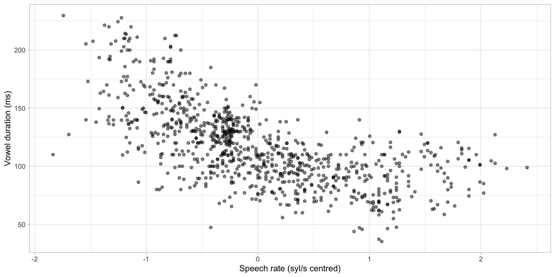
Figure 2: Vowel duration and (centred) speech rate.
Regression model of vowel durations: centred speech rate
\[ \begin{align} dur_i & \sim LogNormal(\mu_i, \sigma)\\ \mu_i & = \beta_0 + \beta_1 \cdot SR_{ctr[i]}\\ \end{align} \]
\(\beta_0\) is the intercept. This is the mean RT when centred speech rate is 0 (i.e. when speech rate is at its mean = NA).
\(\beta_1\) is the slope. This is the change in RT for each unit increase of centred speech rate (i.e for every unit increase of speech rate).
Regression model of vowel durations: code
Regression model: summary
 Family: lognormal
  Links: mu = identity; sigma = identity
Formula: v1_duration ~ 1 + speech_rate_c
   Data: durations (Number of observations: 886)
  Draws: 4 chains, each with iter = 2000; warmup = 1000; thin = 1;
         total post-warmup draws = 4000

Regression Coefficients:
              Estimate Est.Error l-95% CI u-95% CI Rhat Bulk_ESS Tail_ESS
Intercept         4.72      0.01     4.71     4.74 1.00     4388     2452
speech_rate_c    -0.23      0.01    -0.25    -0.22 1.00     4482     2982

Further Distributional Parameters:
      Estimate Est.Error l-95% CI u-95% CI Rhat Bulk_ESS Tail_ESS
sigma     0.22      0.01     0.21     0.23 1.00     3913     2983

Draws were sampled using sampling(NUTS). For each parameter, Bulk_ESS
and Tail_ESS are effective sample size measures, and Rhat is the potential
scale reduction factor on split chains (at convergence, Rhat = 1).
Interpreting the summary
\[ \begin{align} dur_i & \sim LogNormal(\mu_i, \sigma)\\ \mu_i & = \beta_0 + \beta_1 \cdot SR_{ctr[i]}\\ \end{align} \]
                Estimate   Est.Error       Q2.5      Q97.5
Intercept      4.7230357 0.007580906  4.7081901  4.7379128
speech_rate_c -0.2344362 0.009378120 -0.2525304 -0.2157794Interceptis \(\beta_0\): mean duration when speech rate is at mean.speech_rate_cis \(\beta_1\): change in duration for each unit increase of speech rate.
Interpreting the summary: Intercept
                Estimate   Est.Error       Q2.5      Q97.5
Intercept      4.7230357 0.007580906  4.7081901  4.7379128
speech_rate_c -0.2344362 0.009378120 -0.2525304 -0.2157794
The mean logged vowel duration is on average 4.72 (SD = 0.008).
There is a 95% probability that the mean logged vowel duration is between 4.71 and 4.74.
Interpreting the summary: speech_rate_c
                Estimate   Est.Error       Q2.5      Q97.5
Intercept      4.7230357 0.007580906  4.7081901  4.7379128
speech_rate_c -0.2344362 0.009378120 -0.2525304 -0.2157794
The average change in logged vowel duration for each unit increase of speech rate is -0.23 (SD = 0.01).
In other words, for each increase of one syllable per second, the logged vowel duration decreases on average by -0.23.
We can be 95% confident that the decrease in logged duration is between -0.22 and -0.25.
Plotting the model predictions

Figure 3
Posterior predictive checks
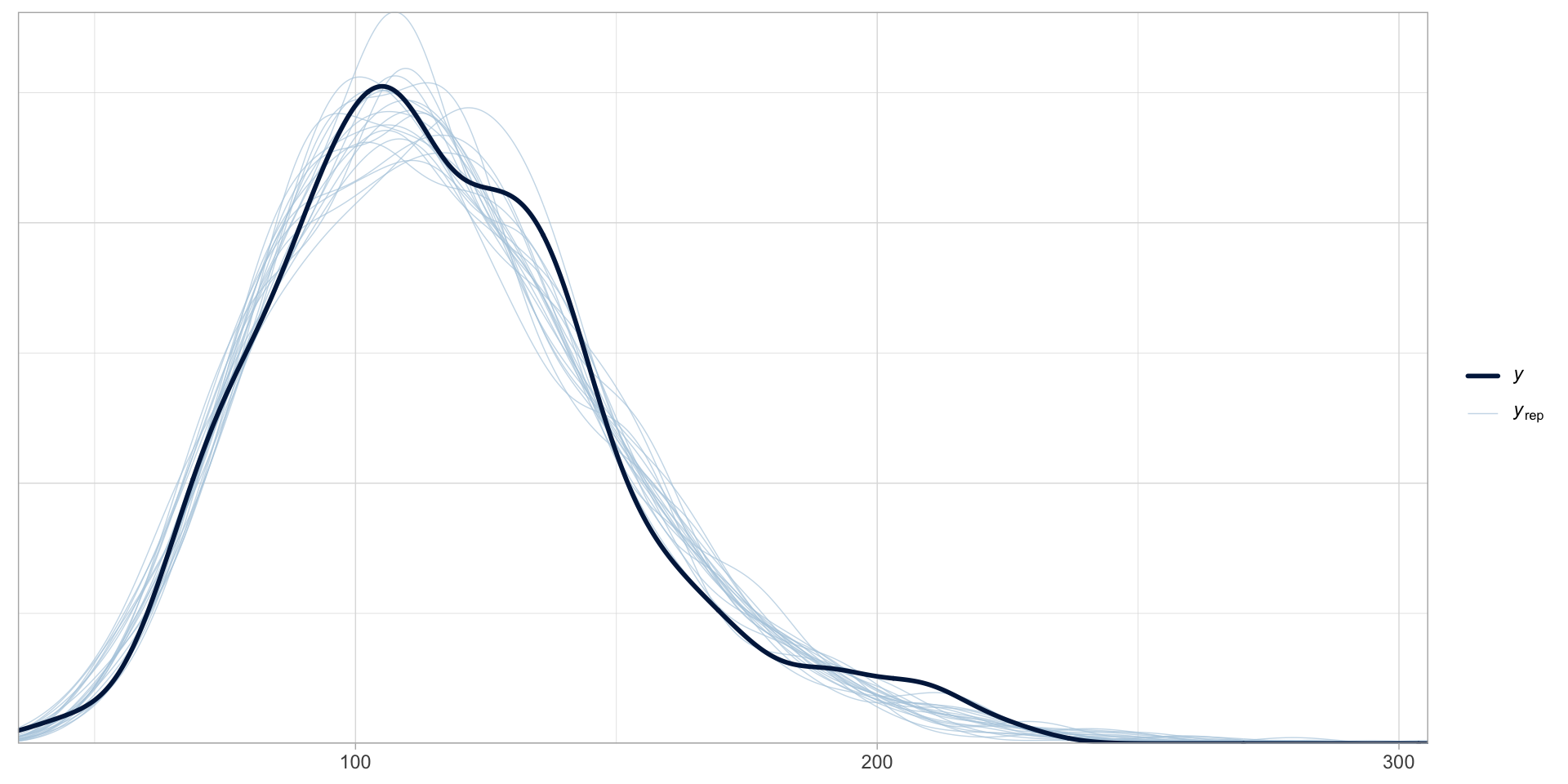
Figure 4: Posterior predictive check plot of dur_sr.
Summary
Regression models are models that use the formula of a line.
A simple regression model with one numeric predictor estimates the line’s intercept (\(beta_0\)) and slope (\(beta_1\)) and the overall standard deviation (\(sigma\)).
\[ \begin{align} y_i & \sim LogNormal(\mu_i, \sigma)\\ \mu_i & = \beta_0 + \beta_1 \cdot x \end{align} \]