02 - Lognormal models

Stefano Coretta

Is a Gaussian model a good choice?

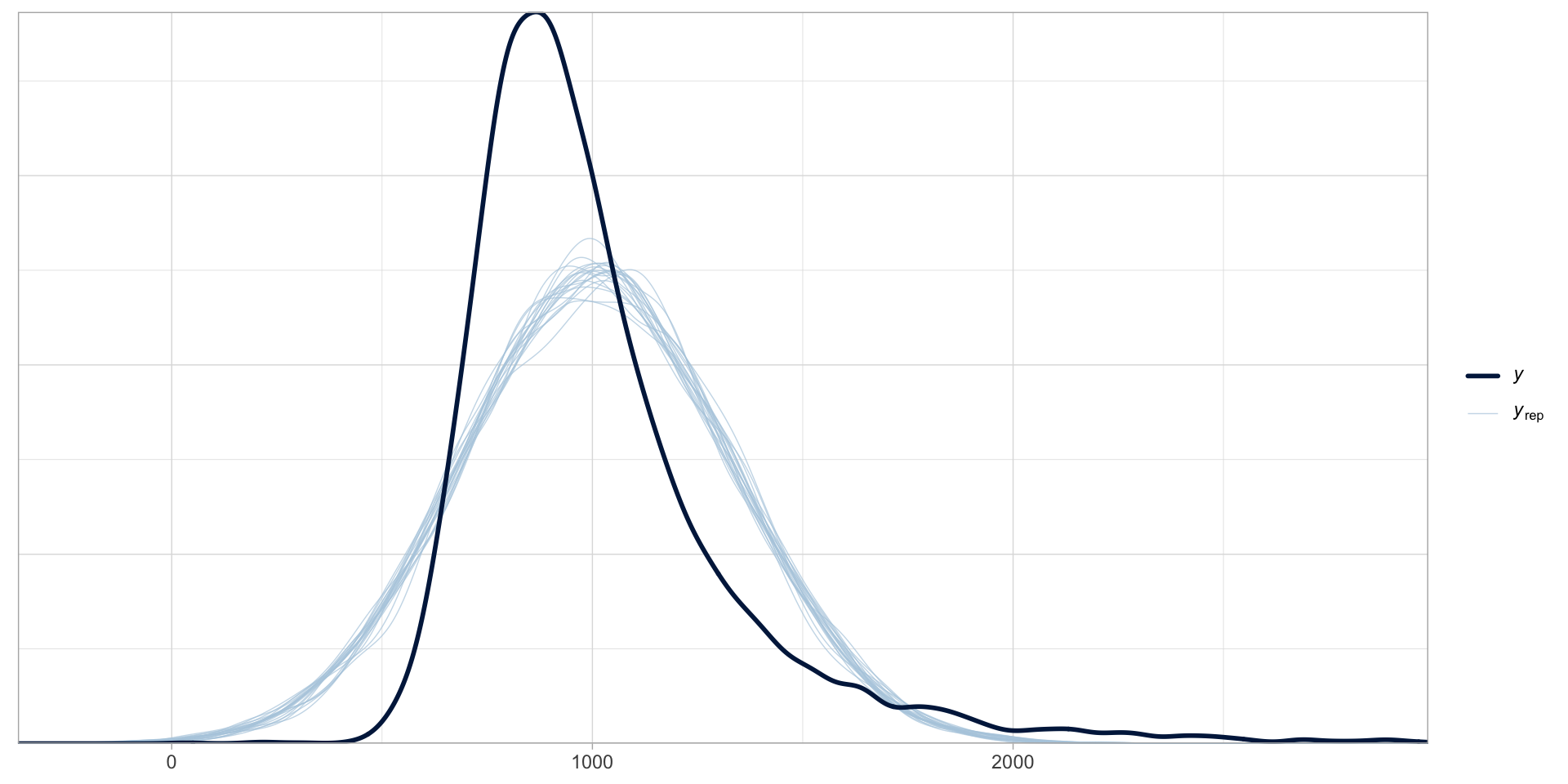
Figure 1: Posterior predictive check plot of rt_gauss.

Gaussian variables are rare…

• Reaction times can only be positive (negative values are excluded).

• Variables that can take only positive numbers (and are continuous) usually follow a log-normal distribution.

The log-normal distribution

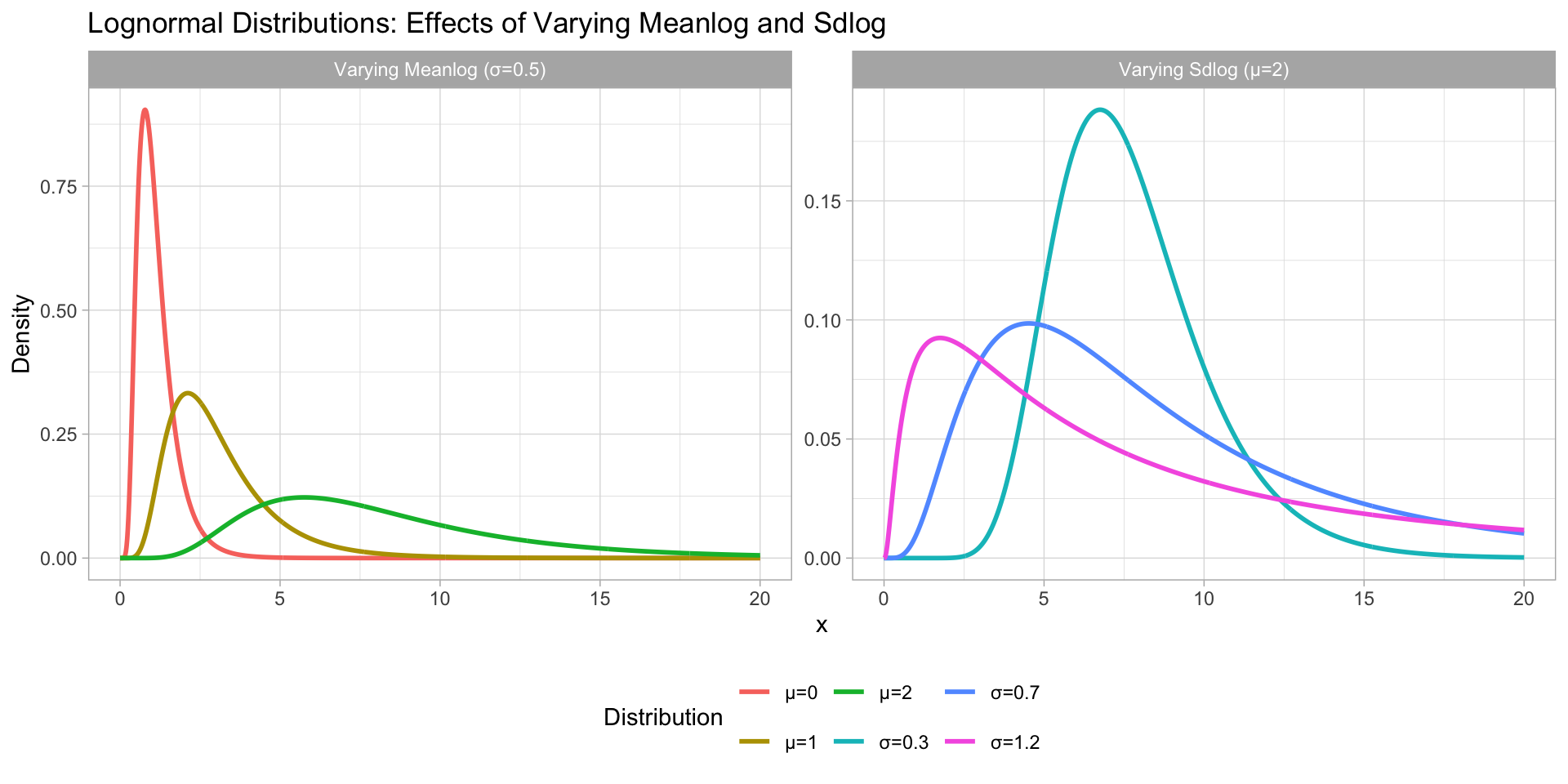
Figure 2: Log-normal distributions with varying mean and SD.

A log-normal model of RTs

\[ \begin{align} RT & \sim LogNormal(\mu, \sigma)\\ \end{align} \]

• RT follow a log-normal distribution with mean \(\mu\) and standard deviation \(\sigma\).

• \(\mu\) and \(sigma\) are the mean and SD of logged RTs.

equivalent to:

\[ \begin{align} log(RT) & \sim Gaussian(\mu, \sigma)\\ \end{align} \]

A log-normal model of RTs: code

rt_logn <- brm(
  RT ~ 1,
  family = lognormal,
  data = mald,
  
  ## Technical stuff
  cores = 4,
  seed = 1032,
  file = "data/cache/rt_logn"
)

A log-normal model of RTs: posterior predictive checks

pp_check(rt_logn, ndraws = 20)

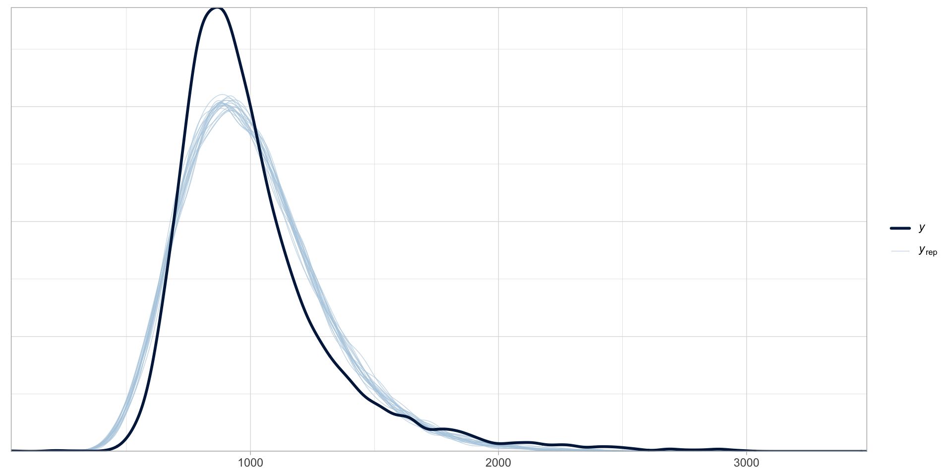
Figure 3

A log-normal model of RTs: summary

summary(rt_logn)

 Family: lognormal 
  Links: mu = identity; sigma = identity 
Formula: RT ~ 1 
   Data: mald (Number of observations: 5000) 
  Draws: 4 chains, each with iter = 2000; warmup = 1000; thin = 1;
         total post-warmup draws = 4000

Regression Coefficients:
          Estimate Est.Error l-95% CI u-95% CI Rhat Bulk_ESS Tail_ESS
Intercept     6.88      0.00     6.87     6.88 1.00     3517     2562

Further Distributional Parameters:
      Estimate Est.Error l-95% CI u-95% CI Rhat Bulk_ESS Tail_ESS
sigma     0.28      0.00     0.27     0.28 1.00     2245     2019

Draws were sampled using sampling(NUTS). For each parameter, Bulk_ESS
and Tail_ESS are effective sample size measures, and Rhat is the potential
scale reduction factor on split chains (at convergence, Rhat = 1).

A log-normal model of RTs: MCMC draws

• The MCMC draws are also called the posterior draws.

• They allow us to construct the posterior probability distribution of each model parameter.

rt_logn_draws <- as_draws_df(rt_logn)

rt_logn_draws

# A draws_df: 1000 iterations, 4 chains, and 5 variables
   b_Intercept sigma Intercept lprior   lp__
1          6.9  0.28       6.9   -3.2 -35094
2          6.9  0.28       6.9   -3.2 -35095
3          6.9  0.27       6.9   -3.1 -35094
4          6.9  0.28       6.9   -3.2 -35094
5          6.9  0.28       6.9   -3.2 -35093
6          6.9  0.28       6.9   -3.2 -35093
7          6.9  0.27       6.9   -3.1 -35095
8          6.9  0.28       6.9   -3.2 -35094
9          6.9  0.28       6.9   -3.2 -35094
10         6.9  0.28       6.9   -3.2 -35096
# ... with 3990 more draws
# ... hidden reserved variables {'.chain', '.iteration', '.draw'}

Plot the MCMC draws: \(\mu\)

rt_logn_draws |> 
  ggplot(aes(b_Intercept)) +
  geom_density(alpha = 0.5, fill = "darkgreen") +
  labs(x = expression(mu~"of RTs (logged)"))

Figure 4: Posterior probability distribution of \(\mu\) of RTs.

Plot the MCMC draws: \(\mu\) (ms)

rt_logn_draws |> 
  ggplot(aes(exp(b_Intercept))) +
  geom_density(alpha = 0.5, fill = "darkgreen") +
  labs(x = expression(mu~"of RTs (ms)"))

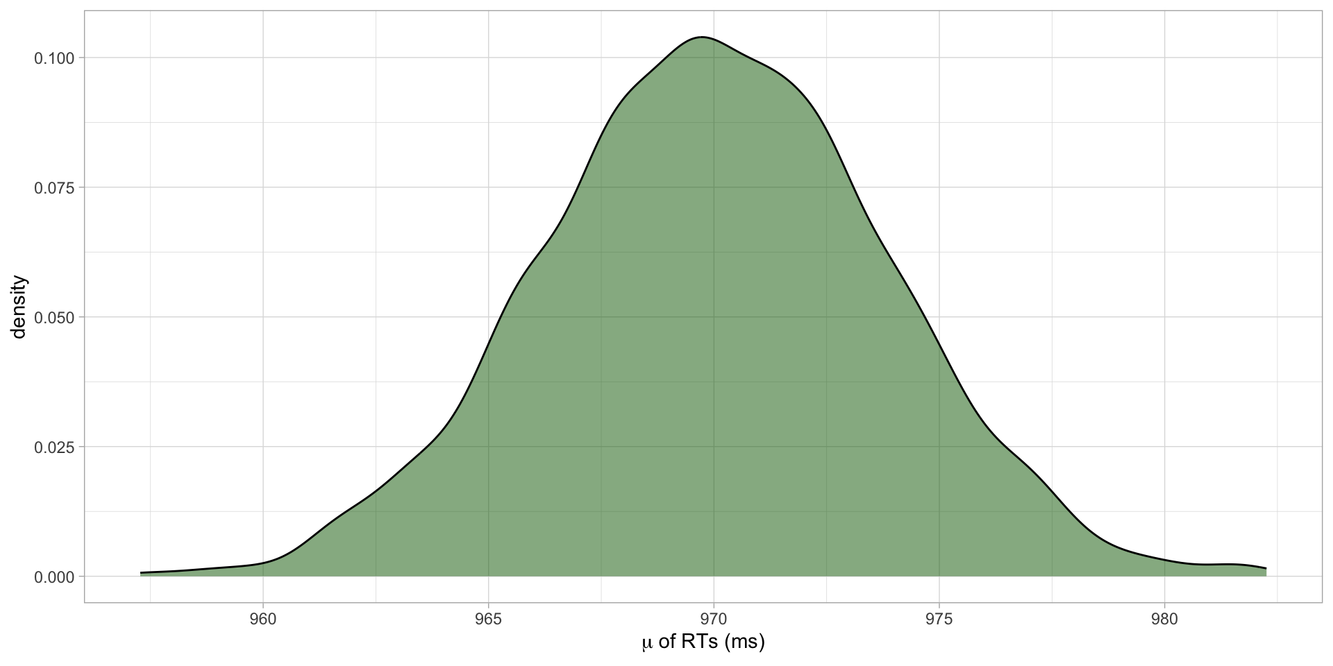
Figure 5: Posterior probability distribution of \(\mu\) of RTs in ms.

Summarise the MCMC draws: \(\mu\)

rt_logn_draws |> 
  summarise(
    mu_mean = round(mean(b_Intercept), 2),
    mu_sd = round(sd(b_Intercept), 3)
  )

# A tibble: 1 × 2
  mu_mean mu_sd
    <dbl> <dbl>
1    6.88 0.004

Summarise the MCMC draws: \(\mu\) (ms)

rt_logn_draws |> 
  summarise(
    mu_mean = round(mean(exp(b_Intercept))),
    mu_sd = round(sd(exp(b_Intercept)))
  )

# A tibble: 1 × 2
  mu_mean mu_sd
    <dbl> <dbl>
1     970     4

• The mean RTs is on average 970 ms (SD = 4).

• Always conditional on the model and the data.

\[ \text{SD}_{\text{natural}} = \sqrt{ \left( e^{\sigma^2} - 1 \right) \cdot e^{2\mu + \sigma^2} } \]

Credible Intervals

• Uncertainty can be quantified with Bayesian Credible Intervals (CrIs).

• A 95% CrI means that we can be 95% confident that the value is within the interval.

Frequentist Confidence Intervals are often wrongly interpreted as Bayesian Credible Intervals (Tan and Tan 2010; Foster 2014; Crooks, Bartel, and Alibali 2019; Gigerenzer, Krauss, and Vitouch 2004; Cassidy et al. 2019).

• There is nothing special about 95%. You should obtain several.

Credible Intervals: higher level = larger width

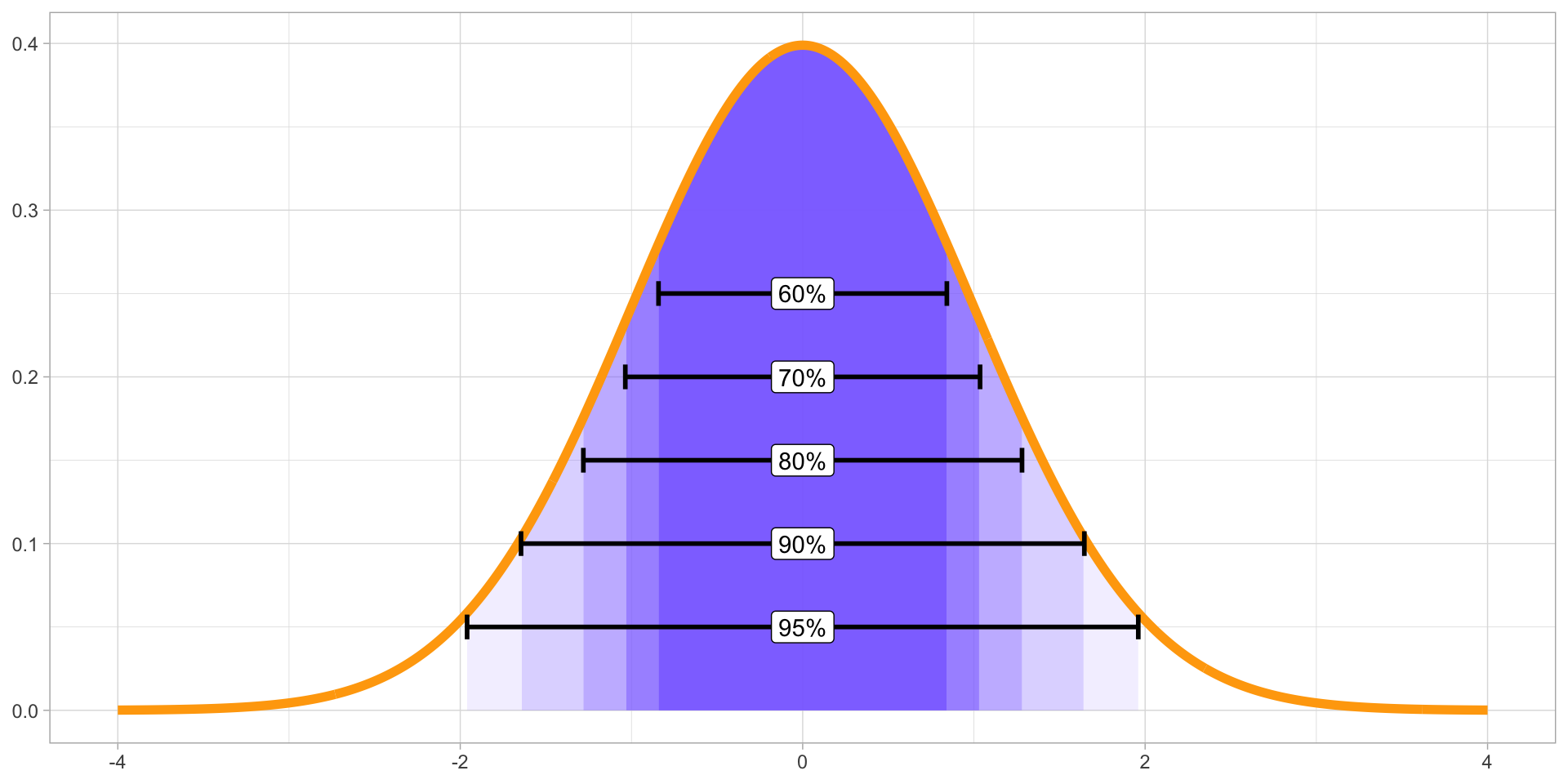
Figure 6: Several quantiles of a Gaussian distribution.

Calculate CrIs

library(posterior)

rt_logn_draws |> 
  mutate(
    mu_ms = exp(b_Intercept)
  ) |> 
  summarise(
    hi_95 = quantile2(mu_ms, probs = 0.025),
    lo_95 = quantile2(mu_ms, probs = 0.975),
    hi_80 = quantile2(mu_ms, probs = 0.1),
    lo_80 = quantile2(mu_ms, probs = 0.9),
    hi_60 = quantile2(mu_ms, probs = 0.2),
    lo_60 = quantile2(mu_ms, probs = 0.8),
  ) |> 
  mutate(across(everything(), round))

# A tibble: 1 × 6
  hi_95 lo_95 hi_80 lo_80 hi_60 lo_60
  <dbl> <dbl> <dbl> <dbl> <dbl> <dbl>
1   962   977   965   975   967   973

Report

We fitted a Bayesian log-normal model of reaction times (RTs) with brms (Bürkner 2017) in R (R Core Team 2025).

According to the model, the mean RT is between 962 and 977 ms, at 95% confidence (in logged ms, \(\beta\) = 6.88, SD = 0.004). At 80% probability, the mean RT is 965-975 ms, while at 60% probability it is 967-973 ms.

Summary

• Gaussian variables are rare.

• Variables that are bounded to positive (real) numbers only usually follow a log-normal distribution. For example reaction times.

• Log-normal models estimate the mean and standard deviation of log-normal variables.

\[ y \sim LogNormal(\mu, \sigma) \]

References

Bürkner, Paul-Christian. 2017. “Brms: An r Package for Bayesian Multilevel Models Using Stan.” Journal of Statistical Software 80 (1): 128. https://doi.org/10.18637/jss.v080.i01.

Cassidy, Scott A., Ralitza Dimova, Benjamin Giguère, Jeffrey R. Spence, and David J. Stanley. 2019. “Failing Grade: 89 Per-Cent of Introduction to Psychology Textbooks That Define/Explain Statistical Significance Do so Incorrectly.” Advances in Methods and Practices in Psychological Science. https://doi.org/10.1177/2515245919858072.

Crooks, Noelle M., Anna N. Bartel, and Martha W. Alibali. 2019. “Conceptual Knowledge of Confidence Intervals in Psychology Undergraduate and Graduate Students.” Statistics Education Research Journal 18 (1): 46–62. https://doi.org/10.52041/serj.v18i1.149.

Foster, Colin. 2014. “Confidence Trick: The Interpretation of Confidence Intervals.” Canadian Journal of Science, Mathematics and Technology Education 14 (1): 2334. https://doi.org/10.1080/14926156.2014.874615.

Gigerenzer, Gerd, Stefan Krauss, and Oliver Vitouch. 2004. “The Null Ritual. What You Always Wanted to Know about Significance Testing but Were Afraid to Ask.” In, 391408.

R Core Team. 2025. R: A Language and Environment for Statistical Computing [Version 4.5.0].

Tan, Sze Huey, and Say Beng Tan. 2010. “The Correct Interpretation of Confidence Intervals.” Proceedings of Singapore Healthcare 19 (3): 276278. https://doi.org/10.1177/201010581001900316.